In this post, I will introduce the small world property of complex networks. Besides tidyverse, patchwork and kableExtra to handle data and to present tables and graphs, I will be using igraphdata to get a sample of the US airport network, and tidygraph and ggraph to handle network data.
library(tidygraph)
library(ggraph)
library(igraphdata)
library(tidyverse)
library(patchwork)
library(kableExtra)
Behind the concept of small-world networks (Watts & Strogatz, 1998), lies the observation that the global and local properties of real world networks are in a middle ground between regular networks and random networks. Watts and Strogatz used as global property the characteristic path length, and as local property the average clustering coefficient. Let’s describe these two properties, and see how to calculate them.
Characteristic Path Length
In an unewighted graph, the distance between two nodes is equal to the minimum number of edges required to reach the second node fromt the first. The characteristic path lenght or average shortest path length \(L\) of a network is equal to the average value of distances between network nodes. For an undirected graph is equal to:
\[ L = \frac{2}{N\left(N-1\right)} \sum_{i>j} d_{ij}\]
If two nodes of the network are disconnected, the distance between these nodes is infinite, so \(L\) diverges to infinity.
Average Clustering Coefficient
The clustering coefficient measures the cliqueness of a node, that is, the number of edges between the neighbours of a node. If the number of neighbors of a node \(i\) is equal to its degree \(k_i\) and the number of edges between neighbours of \(i\) is equal to \(e_i\), the local clustering coefficient is equal to:
\[c_i. = \frac{2e_i}{k_i\left(k_i - 1\right)}\]
By definition, \(c_i\) is set to zero for nodees with only one neighbour.
and the average clustering coefficient \(C\) is equal to the mean \(c_i\) across network nodes:
\[C = \frac{1}{N} \sum_{i=1}^N c_i\]
Let’s illustrate clustering coefficient with a star graph (left) and a clustered star star_clust graph (right):
star_plot <- function(table){

  g <- as_tbl_graph(table)

  ggraph(g, layout = "star") +
    geom_node_text(aes(label = name), size = 7) +
    geom_edge_link(alpha = 0.5,
                   start_cap = circle(3, "mm"), end_cap = circle(3, "mm"),
                   edge_width = 2) +
    theme_graph()

}

star <- data.frame(org = rep(1, 6),
               dst = 2:7)

star_clust <- data.frame(org = c(rep(1,6), 2, 3, 2),
                     dst = c(2:7, 3, 4, 4))

star_plot(star) + star_plot(star_clust)
## Warning: Using the `size` aesthetic in this geom was deprecated in ggplot2 3.4.0.
## ℹ Please use `linewidth` in the `default_aes` field and elsewhere instead.
## This warning is displayed once every 8 hours.
## Call `lifecycle::last_lifecycle_warnings()` to see where this warning was
## generated.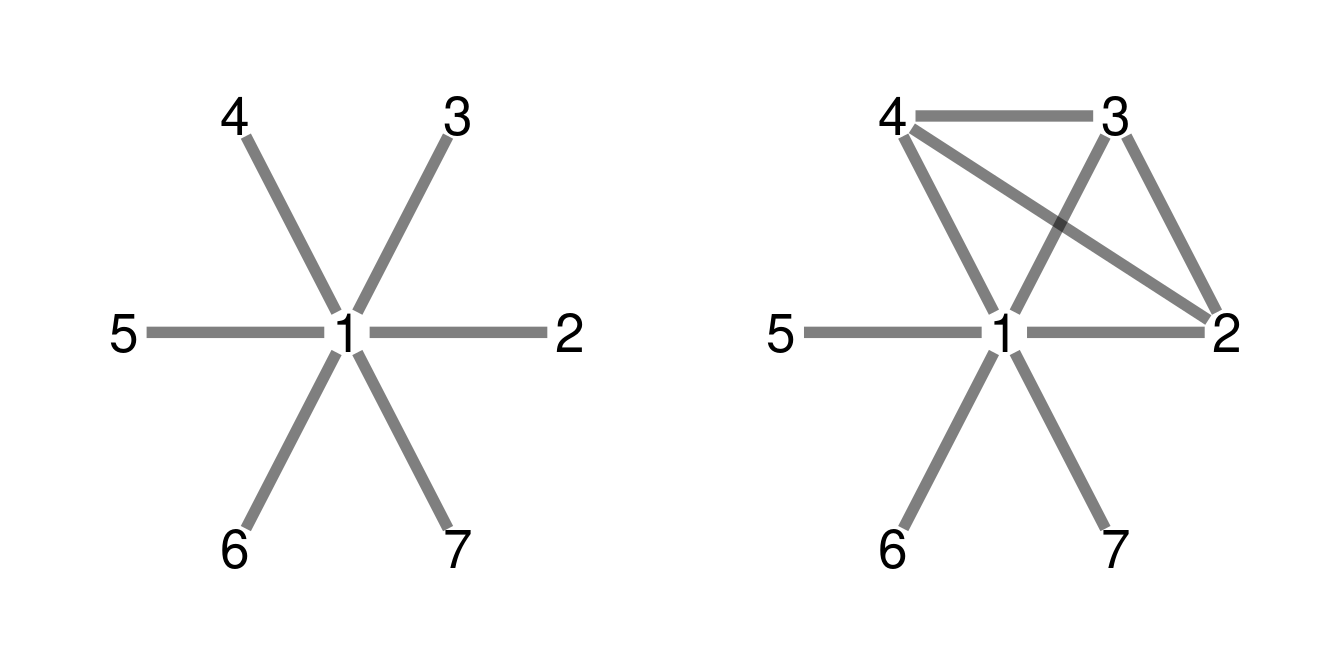
In the star graph, there are no edges between the neighbours of any node. For nodes 2 to 7 \(c_i\) is zer because they have only one neighbour. For node 1 \(c_i\) is also zero as there is no edges between nodes 2 through 7.
For star_clust, \(c_i = 0\) for nodes 5 to 7. As node 1 has six neighbours, and there are three edges between nodes to 2 to 7, we have:
\[c_1 = \frac{2 \times 3}{6 \times 5} = 0.2\]
And for nodes 2 to 4 \(c_i = 1\) as their neighbourhoods are fully connected. Therefore, for star_clust \(C = 0.457\).
The Small-World Property of Regular and Random Networks
Regular and random networks have distinct behaviors regarding the evolution of \(L\) and \(C\) with network size \(N\):
- In random networks, characteristic path length grows logartihmically with \(N\), \(L \sim ln N / ln \langle k \rangle\), where \(\langle k \rangle\) is the average degree. Clustering coefficient vanishes with size \(C \sim \langle k \rangle/ N\).
- In regular networks, characteristic path length grows linearly with \(N\) while clustering coefficient remains constant with \(N\).
meas_lattice <- function(av_degree, size){

  lattice <- play_smallworld(n_dim = 1, dim_size = size, order = round(av_degree/2), p = 0)

  meas <- lattice |>
    activate(nodes) |>
    mutate(L = graph_mean_dist(),
           C = local_transitivity()) |>
    as_tibble() |>
    summarise(across(everything(), mean))

  meas <- meas |>
    mutate(N = size,
           graph = "regular") |>
    select(graph, N, L, C)

  return(meas)

}

meas_random <- function(av_degree, size, sample){

  m <- map_dfr(1:sample, ~{
    random <- play_erdos_renyi(n = size, m = size*av_degree/2, directed = FALSE)

    t <- random |>
      activate(nodes) |>
      mutate(L = graph_mean_dist(),
             C = local_transitivity()) |>
      as_tibble() |>
      summarise(across(everything(), mean))

  })

  meas <- m |>
    summarise(across(everything(), mean)) |>
    mutate(N = size,
           graph = "random") |>
    select(graph, N, L, C)

  return(meas)
}

Ns <- seq(100, 1000, by = 100)

table_lattice <- map_dfr(Ns, ~ meas_lattice(av_degree = 4, size = .))
table_random <- map_dfr(Ns, ~meas_random(av_degree = 4, size = ., sample = 10))

table_all <- rbind(table_lattice, table_random)
In the following plot we can see how \(L\) and \(C\) scale with \(N\) for networks of average degree equal to 8. Note the difference of scaling of \(L\) and \(C\) for both graph models, and how \(C\) decreases in random nodes while remains constant in regular nodes.
plotL <- table_all |>
  mutate(graph = fct_relevel(graph, "regular", "random")) |>
  ggplot(aes(N, L)) +
  geom_point() +
  scale_x_continuous(breaks = seq(100, 1000, by = 100)) +
  facet_grid(graph ~  ., scales = "free") +
  theme_bw()

plotC <- table_all |>
  mutate(graph = fct_relevel(graph, "regular", "random")) |>
  ggplot(aes(N, C)) +
  geom_point() +
  scale_x_continuous(breaks = seq(100, 1000, by = 100)) +
  facet_grid(graph ~  ., scales = "free") +
  theme_bw()

plotL + plotC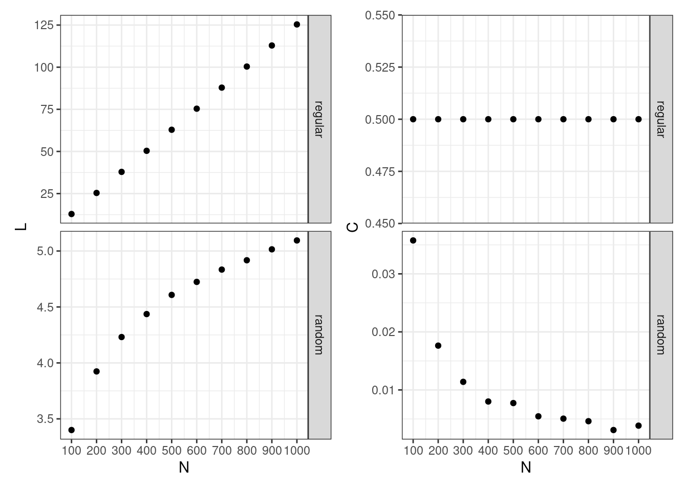
Modelling Small-World Networks
As real-world networks lie somewhere in between regular and random networks, Watts and Strogatz proposed modelling those networks as regular lattices with nodes reconnected at random with a rewiring mechanism.
plot_ws <- function(dim_size, order, p){

  g <- play_smallworld(n_dim = 1, dim_size = dim_size, order = order, p = p)

  ggraph(g, layout = "circle") +
    geom_node_point(size = 2) +
    geom_edge_link(alpha = 0.4) +
    ggtitle(paste0("p = ", p)) +
    theme_graph() +
    theme(plot.title = element_text(hjust = 0.5, size = 10))
}

set.seed(1111)
plot_ws(20, 4, 0) + plot_ws(20, 4, 0.05) + plot_ws(20, 4, 1)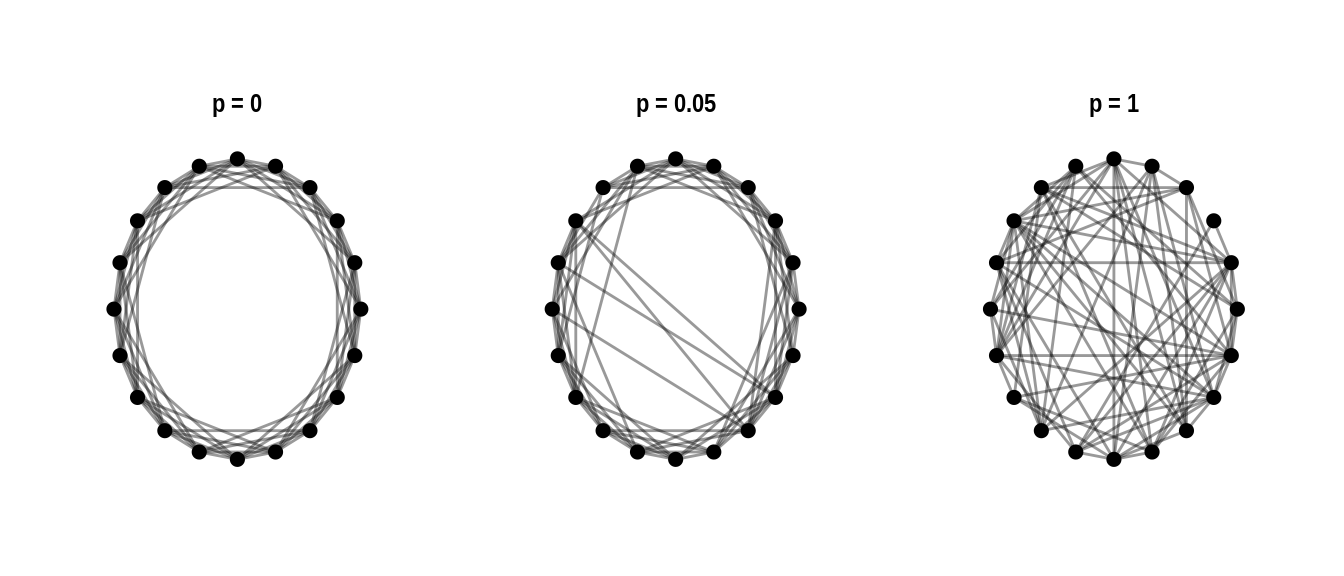
When the probability of rewiring is \(p=0\) we have a regular network, and when \(p=1\) a random network. For intermediate values of \(p\) we have a Watts-Strogatz (WS) network.
For even small values of \(p\), the rewired edges reduce largely \(L\) while maintaining the high value of \(C\) of a regular network. In the following chart, which reproduces the results of the original Watts & Strogatz (1998) paper, we observe the range of values of p with low \(L\) and high \(C\). The values of \(L\) and \(C\) are scaled to the values with \(p=0\).
meas_ws <- function(n, order, p_rewiring){

  g <- play_smallworld(n_dim = 1, dim_size = n, order = order, p = p_rewiring)

  meas <- g |>
    activate(nodes) |>
    mutate(l = graph_mean_dist(),
           c = local_transitivity()) |>
    as_tibble() |>
    summarise(L = mean(l), C = mean(c))

  meas <- meas |>
    mutate(p = p_rewiring) |>
    select(p, L, C)

  return(meas)

}

p <- c(0, rep(10^{seq(-4, 0, length.out = 15)}, 20))

sm_values <- map_dfr(p, ~ meas_ws(n = 1000, order = 5, p_rewiring = .))

scale_sm_values <- sm_values |>
  filter(p == 0)

sm_values |>
  group_by(p) |>
  summarise(across(L:C, mean)) |>
  mutate(L = L/scale_sm_values$L,
         C = C/scale_sm_values$C) |>
  filter(p != 0) |>
  pivot_longer(-p) |>
  ggplot(aes(p, value, color = name)) +
  scale_x_log10() +
  geom_point(size = 2) +
  scale_color_manual(name = "measure", labels = c("C/C(0)", "L/L(0)"), values = c("#FF8000", "#0080FF")) +
  theme_minimal() +
  labs(y = element_blank()) +
  theme(legend.position = c(0.9, 0.9))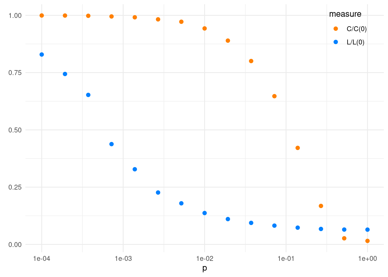
The Small-World Property of Real World Networks
Let’s examine how \(L\) and \(C\) behave in the USairports real-world network from the igraphdata package. To avoid divergence of \(L\), I have examined the largest connected component of this network.
data("USairports")

us_airports <- as_tbl_graph(USairports)

us_airports <- us_airports |>
  convert(to_simple)

us_airports <- us_airports |>
  activate(nodes) |>
  mutate(comp = group_components(),
         d = centrality_degree())

us_airports_lcc <- us_airports |>
  convert(to_subgraph, comp == 1, d > 0)

meas_us_airports_lcc <- us_airports_lcc |>
  activate(nodes) |>
  mutate(N = graph_order(),
         E = graph_size(),
         L = graph_mean_dist(),
         C = local_transitivity()) |>
  as_tibble() |>
  select(N:C) |>
  summarise(across(everything(), mean)) |>
  mutate(graph = "US airports") |>
  relocate(graph)

meas_us_airports_lcc |>
  kbl(digits = 3) |>
kable_styling(full_width = FALSE)| graph | N | E | L | C |
|---|---|---|---|---|
| US airports | 740 | 8215 | 3.52 | 0.554 |
The behaviour of this real-world network is in a middle ground: it has a value of C similar to a regular graph, and a value of L similar to a random graph. This is the small-world property of real world networks: a low characteristic path length and a high clustering coefficient. To evaluate if a network has the small-world property, it is common to compare its values of L and C with a random graph of the same value of nodes and edges. In this case we have:
meas_usairp_random <- map_dfr(1:10, ~ {
  g <- play_erdos_renyi(n = meas_us_airports_lcc$N, m = meas_us_airports_lcc$E, directed = FALSE)
meas <- g |>
  activate(nodes) |>
    mutate(N = graph_order(),
         E = graph_size(),
         L = graph_mean_dist(),
         C = local_transitivity()) |>
  as_tibble()
})

av_meas_usairp_random <- meas_usairp_random |>
  summarise(across(everything(), mean)) |>
  mutate(graph = "random") |>
  relocate(graph)

ws_airp <- rbind(meas_us_airports_lcc, av_meas_usairp_random)

ws_airp |>
    kbl(digits = 3) |>
kable_styling(full_width = FALSE)| graph | N | E | L | C |
|---|---|---|---|---|
| US airports | 740 | 8215 | 3.520 | 0.554 |
| random | 740 | 8215 | 2.468 | 0.030 |
While the values of \(L\) for both graphs are of the same order of magnitude, the value of \(C\) of the random newtwork is much smaller. Therefore, we can confirm that the US airport network has the small-world property.
Modelling the Small-World Property
The WS model is a network model that reproduces the small-world network behaviour of real networks, but that does not reproduce the heterogeneous degree distribution modelled by Barabási-Albert (BA) networks. So real-word networks:
- Have the small-world property as WS network models.
- Have a heterogeneous degree distribution similar to BA models.
References
- Watts, D. J. & Strogatz, S. H. (1998). Collective dynamics of “small-world” networks. Nature, 393(6684), 440–442. https://doi.org/10.1038/30918
Session Info
## R version 4.3.1 (2023-06-16)
## Platform: x86_64-pc-linux-gnu (64-bit)
## Running under: Linux Mint 21.1
##
## Matrix products: default
## BLAS:   /usr/lib/x86_64-linux-gnu/blas/libblas.so.3.10.0
## LAPACK: /usr/lib/x86_64-linux-gnu/lapack/liblapack.so.3.10.0
##
## locale:
##  [1] LC_CTYPE=es_ES.UTF-8       LC_NUMERIC=C
##  [3] LC_TIME=es_ES.UTF-8        LC_COLLATE=es_ES.UTF-8
##  [5] LC_MONETARY=es_ES.UTF-8    LC_MESSAGES=es_ES.UTF-8
##  [7] LC_PAPER=es_ES.UTF-8       LC_NAME=C
##  [9] LC_ADDRESS=C               LC_TELEPHONE=C
## [11] LC_MEASUREMENT=es_ES.UTF-8 LC_IDENTIFICATION=C
##
## time zone: Europe/Madrid
## tzcode source: system (glibc)
##
## attached base packages:
## [1] stats     graphics  grDevices utils     datasets  methods   base
##
## other attached packages:
##  [1] kableExtra_1.3.4 patchwork_1.1.2  lubridate_1.9.2  forcats_1.0.0
##  [5] stringr_1.5.0    dplyr_1.1.2      purrr_1.0.1      readr_2.1.4
##  [9] tidyr_1.3.0      tibble_3.2.1     tidyverse_2.0.0  igraphdata_1.0.1
## [13] ggraph_2.1.0     ggplot2_3.4.2    tidygraph_1.2.3
##
## loaded via a namespace (and not attached):
##  [1] gtable_0.3.3       xfun_0.39          bslib_0.5.0        ggrepel_0.9.3
##  [5] tzdb_0.3.0         vctrs_0.6.2        tools_4.3.1        generics_0.1.3
##  [9] fansi_1.0.4        highr_0.10         pkgconfig_2.0.3    webshot_0.5.4
## [13] lifecycle_1.0.3    compiler_4.3.1     farver_2.1.1       munsell_0.5.0
## [17] ggforce_0.4.1      graphlayouts_0.8.4 htmltools_0.5.5    sass_0.4.5
## [21] yaml_2.3.7         crayon_1.5.2       pillar_1.9.0       jquerylib_0.1.4
## [25] MASS_7.3-60        cachem_1.0.7       viridis_0.6.2      tidyselect_1.2.0
## [29] rvest_1.0.3        digest_0.6.31      stringi_1.7.12     bookdown_0.33
## [33] labeling_0.4.2     polyclip_1.10-4    fastmap_1.1.1      grid_4.3.1
## [37] colorspace_2.1-0   cli_3.6.1          magrittr_2.0.3     utf8_1.2.3
## [41] withr_2.5.0        scales_1.2.1       timechange_0.2.0   rmarkdown_2.21
## [45] httr_1.4.5         igraph_1.4.2       gridExtra_2.3      blogdown_1.16
## [49] hms_1.1.3          evaluate_0.20      knitr_1.42         viridisLite_0.4.1
## [53] rlang_1.1.0        Rcpp_1.0.10        glue_1.6.2         xml2_1.3.4
## [57] tweenr_2.0.2       svglite_2.1.1      rstudioapi_0.14    jsonlite_1.8.4
## [61] R6_2.5.1           systemfonts_1.0.4