Getting and cleaning data is one of the most time-consuming activities in data analysis. This job consists of acquiring data from an unstructured source (if you prefer, from a source with maintainers with different ideas of what a structured dataset is) and transforming it into a (correctly) structured dataset. Paraphrasing Tolstoy, we can say that “structured datasets are all alike; every unstructured dataset is unstructured in its own way”.
In this post, I will present how I have retrieved sunrise (orto in Spanish) and sunset (ocaso in Spanish) hours in Barcelona during 2019. Data is publicly available as a text file from the following link:
https://cdn.mitma.gob.es/portal-web-drupal/salidapuestasol/2019/Barcelona-2019.txt
Let’s save the link in a R variable.
url_oo <- "https://cdn.mitma.gob.es/portal-web-drupal/salidapuestasol/2019/Barcelona-2019.txt"In this post, I will rely on the powers of the tidyverse.
library(tidyverse)Among the packages loaded in the above instruction is the stringr package, which will be very useful in this job.
Looking at Data
We can take a look at the data using readLines. This function parses a text file, so that each line is the component of a vector. As all reading functions from R, input can be a location in your computer or a link to a remote resource.
oo <- readLines(url_oo)
oo
## [1] "BARCELONA SALIDA Y PUESTA DE SOL PARA 2019 Observatorio Astron\xf3mico Nacional"
## [2] "Latitud y longitud: 41 23 7, + 2 10 39 Instituto Geogr\xe1fico Nacional"
## [3] "A\xf1o 2019 Hora oficial en la pen\xednsula y Baleares Ministerio de Fomento, Espa\xf1a"
## [4] ""
## [5] "Dia Enero Febrero Marzo Abril Mayo Junio Julio Agosto Septiem. Octubre Noviemb. Diciemb."
## [6] " Ort Ocas Ort Ocas Ort Ocas Ort Ocas Ort Ocas Ort Ocas Ort Ocas Ort Ocas Ort Ocas Ort Ocas Ort Ocas Ort Ocas"
## [7] " h m h m h m h m h m h m h m h m h m h m h m h m h m h m h m h m h m h m h m h m h m h m h m h m"
## [8] " 1 817 1732 803 1807 726 1841 735 2016 649 2048 620 2118 621 2129 646 2109 717 2025 748 1934 722 1747 757 1723"
## [9] " 2 817 1733 802 1808 725 1843 734 2017 648 2049 620 2119 622 2129 647 2108 718 2023 749 1932 723 1746 758 1722"
## [10] " 3 818 1734 801 1810 723 1844 732 2018 647 2051 620 2120 622 2128 648 2107 719 2022 750 1930 725 1744 759 1722"
## [11] " 4 818 1735 800 1811 722 1845 730 2019 645 2052 619 2120 623 2128 649 2105 720 2020 751 1929 726 1743 800 1722"
## [12] " 5 818 1736 759 1812 720 1846 729 2020 644 2053 619 2121 624 2128 650 2104 721 2018 752 1927 727 1742 801 1722"
## [13] " 6 817 1737 758 1813 719 1847 727 2021 643 2054 619 2122 624 2128 651 2103 722 2017 753 1925 728 1741 802 1722"
## [14] " 7 817 1738 757 1815 717 1848 725 2023 642 2055 618 2122 625 2127 652 2102 723 2015 754 1924 729 1740 803 1722"
## [15] " 8 817 1739 756 1816 715 1850 724 2024 640 2056 618 2123 625 2127 653 2100 724 2013 755 1922 731 1739 804 1722"
## [16] " 9 817 1740 754 1817 714 1851 722 2025 639 2057 618 2123 626 2127 654 2059 725 2012 756 1921 732 1738 805 1722"
## [17] "10 817 1741 753 1818 712 1852 720 2026 638 2058 618 2124 627 2126 655 2058 726 2010 757 1919 733 1737 806 1722"
## [18] "11 817 1742 752 1820 710 1853 719 2027 637 2059 617 2125 628 2126 656 2057 727 2008 758 1917 734 1736 807 1722"
## [19] "12 816 1743 751 1821 709 1854 717 2028 636 2100 617 2125 628 2125 657 2055 728 2006 759 1916 736 1735 808 1722"
## [20] "13 816 1744 749 1822 707 1855 716 2029 635 2101 617 2125 629 2125 658 2054 729 2005 800 1914 737 1734 808 1722"
## [21] "14 816 1745 748 1823 705 1856 714 2030 634 2102 617 2126 630 2124 659 2052 730 2003 801 1913 738 1733 809 1722"
## [22] "15 815 1746 747 1825 704 1857 712 2031 633 2103 617 2126 631 2124 700 2051 731 2001 803 1911 739 1732 810 1722"
## [23] "16 815 1747 745 1826 702 1859 711 2032 632 2104 617 2127 631 2123 701 2050 732 2000 804 1909 740 1731 811 1723"
## [24] "17 814 1749 744 1827 700 1900 709 2033 631 2105 617 2127 632 2122 702 2048 733 1958 805 1908 742 1730 811 1723"
## [25] "18 814 1750 743 1828 659 1901 708 2034 630 2106 617 2127 633 2122 703 2047 734 1956 806 1906 743 1730 812 1723"
## [26] "19 813 1751 741 1830 657 1902 706 2035 629 2107 618 2128 634 2121 704 2045 735 1954 807 1905 744 1729 813 1724"
## [27] "20 813 1752 740 1831 655 1903 705 2037 628 2108 618 2128 635 2120 705 2044 736 1953 808 1903 745 1728 813 1724"
## [28] "21 812 1753 738 1832 654 1904 703 2038 628 2109 618 2128 636 2119 706 2042 737 1951 809 1902 746 1727 814 1725"
## [29] "22 811 1755 737 1833 652 1905 702 2039 627 2110 618 2128 636 2119 707 2041 738 1949 811 1900 747 1727 814 1725"
## [30] "23 811 1756 736 1834 650 1906 700 2040 626 2111 618 2129 637 2118 708 2039 739 1948 812 1859 749 1726 815 1726"
## [31] "24 810 1757 734 1836 649 1907 659 2041 625 2112 619 2129 638 2117 709 2038 740 1946 813 1858 750 1726 815 1726"
## [32] "25 809 1758 733 1837 647 1908 657 2042 625 2112 619 2129 639 2116 710 2036 741 1944 814 1856 751 1725 816 1727"
## [33] "26 808 1759 731 1838 645 1910 656 2043 624 2113 619 2129 640 2115 711 2035 742 1942 815 1855 752 1725 816 1728"
## [34] "27 808 1801 730 1839 644 1911 655 2044 623 2114 620 2129 641 2114 712 2033 743 1941 716 1753 753 1724 816 1728"
## [35] "28 807 1802 728 1840 642 1912 653 2045 623 2115 620 2129 642 2113 713 2031 744 1939 718 1752 754 1724 817 1729"
## [36] "29 806 1803 640 1913 652 2046 622 2116 620 2129 643 2112 714 2030 745 1937 719 1751 755 1723 817 1730"
## [37] "30 805 1804 639 1914 650 2047 621 2117 621 2129 644 2111 715 2028 746 1936 720 1749 756 1723 817 1730"
## [38] "31 804 1806 737 2015 621 2117 645 2110 716 2027 721 1748 817 1731"
## [39] " h m h m h m h m h m h m h m h m h m h m h m h m h m h m h m h m h m h m h m h m h m h m h m h m"
## [40] ""
## [41] "Se ha considerado el horario adelantado desde el \xfaltimo domingo de marzo al \xfaltimo domingo de octubre. Las coordenadas"
## [42] "vienen dadas en grados, minutos y segundos, siendo la longitud positiva al Este y negativa al Oeste del meridiano cero."Taking a look at the results we observe that:
- Data is between lines 8 and 38.
- Column names are useless in this context.
- Sunrise and sunset hours occur in the same positions of each line for all days.
- We can obtain the final position of each sunrise and sunset hour with the
mcharacter in line 7.
To obtain the positions of the m character in line 7, we can use stringr::str_locate_all():
pos_e <- str_locate_all(oo[7], "m")[[1]][ ,1]
pos_e
## [1] 6 11 16 21 26 31 36 41 46 51 56 61 66 71 76 81 86 91 96
## [20] 101 106 111 116 121In pos_e is retrieved the end of each block of data. All sunrise hours have three characters and all sunset have four, so we can find the start of each block doing:
dec <- rep(c(2, 3), 12)
pos_s <- pos_e - dec
pos_s
## [1] 4 8 14 18 24 28 34 38 44 48 54 58 64 68 74 78 84 88 94
## [20] 98 104 108 114 118Therefore, pos_e and pos_s store the positions of each sunrise and sunset hour of each row.
Retrieving the Data
With pos_s and pos_e we can retrieve the data of each row. We can pick each block with stringr::str_sub(). This function picks the values of a string between start and end positions. These can be vectors, so it can separate each value of a row. Let’s illustrate it with the first row:
str_sub(oo[8], pos_s, pos_e)## [1] "817" "1732" "803" "1807" "726" "1841" "735" "2016" "649" "2048"
## [11] "620" "2118" "621" "2129" "646" "2109" "717" "2025" "748" "1934"
## [21] "722" "1747" "757" "1723"We can iterate this expression along rows 8 to 38 of oo and stack all rows together into a data frame. We can do this in one step with purrr::map_dfr(), but we need to name each vector with the same column names. Let’s define the column names setting months as numbers and distinguishing between sunrise and sunset with orto and ocaso. Note how we are using rep() with different arguments to do this.
cn1 <- rep(1:12, each = 2)
cn2 <- rep(c("orto", "ocaso"), times = 12)
cn <- paste(cn1, cn2, sep = "_")
cn
## [1] "1_orto" "1_ocaso" "2_orto" "2_ocaso" "3_orto" "3_ocaso"
## [7] "4_orto" "4_ocaso" "5_orto" "5_ocaso" "6_orto" "6_ocaso"
## [13] "7_orto" "7_ocaso" "8_orto" "8_ocaso" "9_orto" "9_ocaso"
## [19] "10_orto" "10_ocaso" "11_orto" "11_ocaso" "12_orto" "12_ocaso"Now we are ready to arrange the data into a data frame:
table <- map_dfr(oo[8:38], ~ {v <- str_sub(. , pos_s, pos_e)
                              names(v) <- cn
                              return(v)})
Cleaning the Data
Let’s see what we’ve got so far:
table |>
  print(n = Inf)
## # A tibble: 31 × 24
## `1_orto` `1_ocaso` `2_orto` `2_ocaso` `3_orto` `3_ocaso` `4_orto` `4_ocaso`
## <chr> <chr> <chr> <chr> <chr> <chr> <chr> <chr>
## 1 817 1732 "803" "1807" 726 1841 "735" "2016"
## 2 817 1733 "802" "1808" 725 1843 "734" "2017"
## 3 818 1734 "801" "1810" 723 1844 "732" "2018"
## 4 818 1735 "800" "1811" 722 1845 "730" "2019"
## 5 818 1736 "759" "1812" 720 1846 "729" "2020"
## 6 817 1737 "758" "1813" 719 1847 "727" "2021"
## 7 817 1738 "757" "1815" 717 1848 "725" "2023"
## 8 817 1739 "756" "1816" 715 1850 "724" "2024"
## 9 817 1740 "754" "1817" 714 1851 "722" "2025"
## 10 817 1741 "753" "1818" 712 1852 "720" "2026"
## 11 817 1742 "752" "1820" 710 1853 "719" "2027"
## 12 816 1743 "751" "1821" 709 1854 "717" "2028"
## 13 816 1744 "749" "1822" 707 1855 "716" "2029"
## 14 816 1745 "748" "1823" 705 1856 "714" "2030"
## 15 815 1746 "747" "1825" 704 1857 "712" "2031"
## 16 815 1747 "745" "1826" 702 1859 "711" "2032"
## 17 814 1749 "744" "1827" 700 1900 "709" "2033"
## 18 814 1750 "743" "1828" 659 1901 "708" "2034"
## 19 813 1751 "741" "1830" 657 1902 "706" "2035"
## 20 813 1752 "740" "1831" 655 1903 "705" "2037"
## 21 812 1753 "738" "1832" 654 1904 "703" "2038"
## 22 811 1755 "737" "1833" 652 1905 "702" "2039"
## 23 811 1756 "736" "1834" 650 1906 "700" "2040"
## 24 810 1757 "734" "1836" 649 1907 "659" "2041"
## 25 809 1758 "733" "1837" 647 1908 "657" "2042"
## 26 808 1759 "731" "1838" 645 1910 "656" "2043"
## 27 808 1801 "730" "1839" 644 1911 "655" "2044"
## 28 807 1802 "728" "1840" 642 1912 "653" "2045"
## 29 806 1803 " " " " 640 1913 "652" "2046"
## 30 805 1804 " " " " 639 1914 "650" "2047"
## 31 804 1806 " " " " 737 2015 " " " "
## # ℹ 16 more variables: `5_orto` <chr>, `5_ocaso` <chr>, `6_orto` <chr>,
## # `6_ocaso` <chr>, `7_orto` <chr>, `7_ocaso` <chr>, `8_orto` <chr>,
## # `8_ocaso` <chr>, `9_orto` <chr>, `9_ocaso` <chr>, `10_orto` <chr>,
## # `10_ocaso` <chr>, `11_orto` <chr>, `11_ocaso` <chr>, `12_orto` <chr>,
## # `12_ocaso` <chr>There are several problems with this table:
- There are empty spaces with days that do not exist, like 30 of February.
- We need to add a column specifying the day.
- Data is in wide format, and computers need long tables.
- Time is stored as a three- of four-character string.
Let’s tackle those issues step by step. First, let’s put the times that do not exist as NA:
table <- table |>
  mutate(across(everything(), ~ case_when(. == "   " ~ NA,
                                          . == "    " ~ NA,
                                          TRUE ~ .)))
Let’s add the dia column for the day number:
table <- table |>
  mutate(dia = 1:31)
Now we are ready to set the table in long format. In this format, we don’t need to keep the non-existing days, so we remove them with tidyr::drop_na().
table <- table |>
  pivot_longer(-dia, names_to = "var", values_to = "tiempo") |>
  drop_na()
Let’s take a look at the result:
table## # A tibble: 730 × 3
## dia var tiempo
## <int> <chr> <chr>
## 1 1 1_orto 817
## 2 1 1_ocaso 1732
## 3 1 2_orto 803
## 4 1 2_ocaso 1807
## 5 1 3_orto 726
## 6 1 3_ocaso 1841
## 7 1 4_orto 735
## 8 1 4_ocaso 2016
## 9 1 5_orto 649
## 10 1 5_ocaso 2048
## # ℹ 720 more rowsWe can split the values of var with tidyr::separate():
table <- table |>
  separate(var, sep = "_", into = c("mes", "evento"))
table
## # A tibble: 730 × 4
## dia mes evento tiempo
## <int> <chr> <chr> <chr>
## 1 1 1 orto 817
## 2 1 1 ocaso 1732
## 3 1 2 orto 803
## 4 1 2 ocaso 1807
## 5 1 3 orto 726
## 6 1 3 ocaso 1841
## 7 1 4 orto 735
## 8 1 4 ocaso 2016
## 9 1 5 orto 649
## 10 1 5 ocaso 2048
## # ℹ 720 more rowsThere are several ways of picking the hour and minute from this time format. I have chosen to transform it into numeric and to use the rounding floor() function to get the hour hora and get the value of minutes min from h:
table <- table |>
  mutate(tiempo = as.numeric(tiempo),
         hora = floor(tiempo/100),
         min = tiempo - hora*100)
table
## # A tibble: 730 × 6
## dia mes evento tiempo hora min
## <int> <chr> <chr> <dbl> <dbl> <dbl>
## 1 1 1 orto 817 8 17
## 2 1 1 ocaso 1732 17 32
## 3 1 2 orto 803 8 3
## 4 1 2 ocaso 1807 18 7
## 5 1 3 orto 726 7 26
## 6 1 3 ocaso 1841 18 41
## 7 1 4 orto 735 7 35
## 8 1 4 ocaso 2016 20 16
## 9 1 5 orto 649 6 49
## 10 1 5 ocaso 2048 20 48
## # ℹ 720 more rowsFinally, let’s use dplyr::select() to retrieve the columns we need:
table <- table |>
  select(mes, dia, evento, hora, min) |>
  arrange(mes, dia)
table
## # A tibble: 730 × 5
## mes dia evento hora min
## <chr> <int> <chr> <dbl> <dbl>
## 1 1 1 orto 8 17
## 2 1 1 ocaso 17 32
## 3 1 2 orto 8 17
## 4 1 2 ocaso 17 33
## 5 1 3 orto 8 18
## 6 1 3 ocaso 17 34
## 7 1 4 orto 8 18
## 8 1 4 ocaso 17 35
## 9 1 5 orto 8 18
## 10 1 5 ocaso 17 36
## # ℹ 720 more rowsUsing the dataset
The way that the table has been arranged allows using it flexibly. We can collapse the date and time values into a timestamp with lubridate::makedatetime() or create a date with lubridate::makedate() and a time with hms::hms().
As an example, let’s plot sunrise and sunset time for each day.
library(hms)
table |>
  mutate(date = make_date(year = 2019, month = mes, day = dia),
         time = hms(minutes = min, hours = hora)) |>
  ggplot(aes(date, time, color = evento)) +
  geom_line(linewidth = 1) +
  theme_minimal() +
  scale_color_manual(values = c("#FF3333", "#FF9933")) +
  theme(legend.position = "top",
        axis.title = element_blank(),
        plot.title.position = "plot") +
  ggtitle("Sunrise (orto) and sunset (ocaso) in Barcelona (2019)")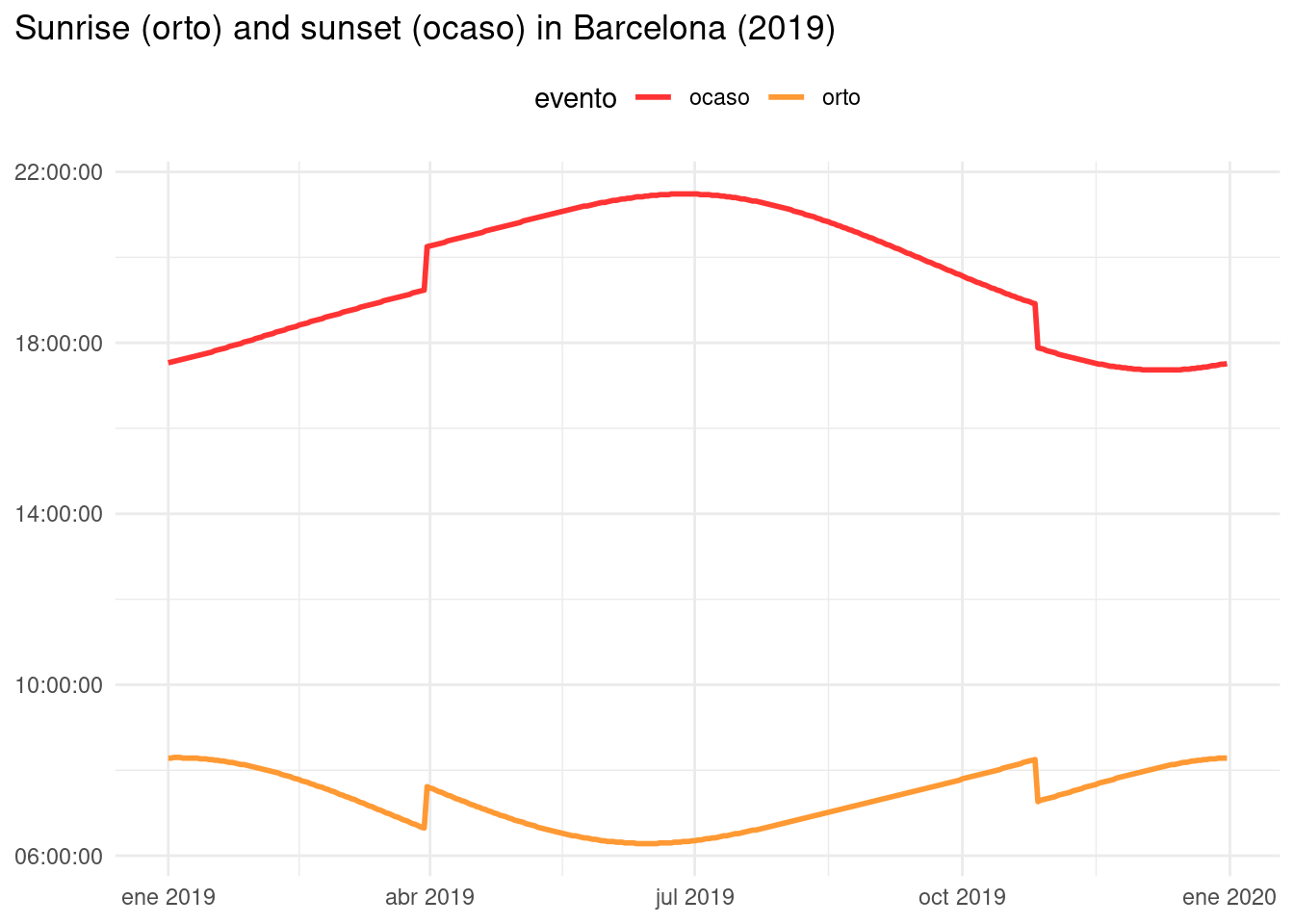
Here we can see the effect of the daylight saving time.
References
- Instituto Geográfico Nacional (2024). Hora, salida y puesta de sol. https://astronomia.ign.es/hora-salidas-y-puestas-de-sol
Session Info
## R version 4.3.2 (2023-10-31)
## Platform: x86_64-pc-linux-gnu (64-bit)
## Running under: Linux Mint 21.1
##
## Matrix products: default
## BLAS:   /usr/lib/x86_64-linux-gnu/blas/libblas.so.3.10.0
## LAPACK: /usr/lib/x86_64-linux-gnu/lapack/liblapack.so.3.10.0
##
## locale:
##  [1] LC_CTYPE=es_ES.UTF-8       LC_NUMERIC=C
##  [3] LC_TIME=es_ES.UTF-8        LC_COLLATE=es_ES.UTF-8
##  [5] LC_MONETARY=es_ES.UTF-8    LC_MESSAGES=es_ES.UTF-8
##  [7] LC_PAPER=es_ES.UTF-8       LC_NAME=C
##  [9] LC_ADDRESS=C               LC_TELEPHONE=C
## [11] LC_MEASUREMENT=es_ES.UTF-8 LC_IDENTIFICATION=C
##
## time zone: Europe/Madrid
## tzcode source: system (glibc)
##
## attached base packages:
## [1] stats     graphics  grDevices utils     datasets  methods   base
##
## other attached packages:
##  [1] hms_1.1.3       lubridate_1.9.3 forcats_1.0.0   stringr_1.5.1
##  [5] dplyr_1.1.4     purrr_1.0.2     readr_2.1.5     tidyr_1.3.0
##  [9] tibble_3.2.1    ggplot2_3.4.4   tidyverse_2.0.0
##
## loaded via a namespace (and not attached):
##  [1] gtable_0.3.3      jsonlite_1.8.8    highr_0.10        compiler_4.3.2
##  [5] tidyselect_1.2.0  jquerylib_0.1.4   scales_1.2.1      yaml_2.3.7
##  [9] fastmap_1.1.1     R6_2.5.1          labeling_0.4.2    generics_0.1.3
## [13] knitr_1.42        bookdown_0.33     munsell_0.5.0     tzdb_0.3.0
## [17] bslib_0.5.0       pillar_1.9.0      rlang_1.1.3       utf8_1.2.3
## [21] stringi_1.7.12    cachem_1.0.7      xfun_0.39         sass_0.4.5
## [25] timechange_0.2.0  cli_3.6.1         withr_2.5.0       magrittr_2.0.3
## [29] digest_0.6.31     grid_4.3.2        rstudioapi_0.15.0 lifecycle_1.0.3
## [33] vctrs_0.6.4       evaluate_0.20     glue_1.6.2        farver_2.1.1
## [37] blogdown_1.16     fansi_1.0.4       colorspace_2.1-0  rmarkdown_2.21
## [41] tools_4.3.2       pkgconfig_2.0.3   htmltools_0.5.5