The genetic algorithm (GA) is a population-based metaheuristic based on the process of natural selection. As living organisms improve its fitness with the environment through evolution, genetic algorithms improve the fitness of each generation of a population of solutions.
To define a genetic algorithm for a specific problem, we need to encode solutions in a suitable way. This encoding is the genotype of the solution. In this post, I will introduce genetic algorithms using permutative encoding, using the travelling salesman problem (TSP) as an example.
In a genetic algorithm, a set of candidate solutions (population) goes through the following processes in each iteration or generation:
- Selection. The solutions of a population need to have a good value of fitness, and also preserve a reasonable degree of diversity. The most popular selection strategy is tournament selection. It consists of selecting a set of solutions at random, and keep the solution with better fitness value.
- Crossover. With crossover, we obtain new solutions combining elements of two or more solutions. The most popular crossover operators for permutative encoding are order crossover (OX) or partial matching crossover (PMX). We can decide to pass to the next generation the solutions obtain through selection or combine them with the crossover operator according to a probability of crossover.
- Mutation. Before going to the next generation, each solution can be altered with a mutation operator, according to a probability of mutation. For the TSP, a mutation operator can be inverting a part of the solution. This is equivalent to applying a 2-opt operator.
In addition to these three processes, there are other elements of the genetic algorithm that can improve its effectiveness.
- Seeding. With seeding, we include in the starting population solutions not obtained at random. A possible seeding strategy can be including a solution obtained with a constructive heuristic such as the nearest neighbour.
- Elitism. With elitism, we pass one or more of the bests solutions of the present generation straight to the next.
Genetic algorithms admit a great diversity of operators. In this post, I will present a specific implementation of a genetic algorithm for the travelling salesman problem.
The code of the algorithm can be retrieved from a Github gist:
devtools::source_gist("https://gist.github.com/jmsallan/1d284ccc9734cc501c2400517d798cfd")## ℹ Sourcing gist "1d284ccc9734cc501c2400517d798cfd"
## ℹ SHA-1 hash of file is "84b6bae29aed049fef1da17b9b873ef75ee00533"I will be using the gr12 and gr24 instances from TSPLIB:
load("gr_instances.RData")And finally I will use the tidyverse mainly for plotting:
library(tidyverse)Selection
I will use tournament selection as selection operator. In this operator, to select a solution we obtain s elements of the population randomly, and the solution with the best fitness is retained. The higher the value of s, the higher the selection pressure, that is, the higher the probability of selecting elements of good fitness. Here I will use s = 6, corresponding to a high selection pressure.
Crossover
I will use the order crossover (OX) operator. This is implemented with the ox_crossover() function. It takes as input two solutions, and as output two new solutions (offspring) obtained as follows.
- The function selects two points
startandendat random between 2 andn-1, beingnthe number of nodes. - The first offspring inherits the sequence
start:endfrom the first input. The rest of the solution is obtained inserting in order the elements of the second input not included in the sequence. - The second offspring has the
start:endsequence of the second output, and the ordered elements not included in the sequence of the first output.
Let’s see an example of application of the crossover operator. Let’s obtain two possible solutions of a problem of size n = 15.
set.seed(1313)
p1 <- c(1, sample(2:15, 14))
p2 <- c(1, sample(2:15, 14))
p1
## [1] 1 4 13 7 15 2 5 11 8 3 14 6 10 12 9p2## [1] 1 7 11 5 8 10 15 9 4 2 14 12 13 3 6Let’s apply the crossover operator to these two solutions:
set.seed(55)
ox_crossover(p1, p2, 15)
## $sibling1
## [1] 1 7 10 9 15 2 5 11 8 3 14 4 12 13 6
##
## $sibling2
## [1] 1 13 7 5 8 10 15 9 4 2 14 11 3 6 12Let’s see how sibling1 is obtained. It takes the sequence from 5 to 11 from p1:
And then selects the elements of p2 not included in the sequence:
The resulting offspring is:
Mutation
The selected mutation operator is the inversion. It consists of inverting a sequence between 3 and n. This is implemented with the inv_mutation() function. Let’s see how it works mutating p1.
set.seed(44)
p1
## [1] 1 4 13 7 15 2 5 11 8 3 14 6 10 12 9inv_mutation(p1, 15)## [1] 1 4 10 6 14 3 8 11 5 2 15 7 13 12 9In this case, the function has inverted the sequence between 3 and 13:
Applying the algorithm to gr24
Let’s apply the algorithm to gr24, an instance from TSPLIB of 24 nodes. The optimal value of this instance is:
tsp_dist(gr24$D, gr24$opt.tour)## [1] 1272Let’s pick a population size of 120. We know that we can obtain the optimum with tabu search with 3,1500 evaluations of the objective function, so we will set 31500/120 ~ 263 generations for the genetic algorithm. Let’s set the probability of crossover to 0.8 and the probability of mutation to 0.4.
set.seed(11)
ga_gr24 <- ga_tsp(instance = gr24$D, selection = "tournament",
                  crossover = "ox", mutation = "inv", npop = 120, max_iter = 263,
                  pcross = 0.8, pmut = 0.4, elitist = TRUE, seed = TRUE)
The algorithm achieves a solution close to the optimum:
ga_gr24$fit## [1] 1289To track the evolution of the algorithm, I am plotting:
- The
bestsolution obtained. - The best solution of the iteration
iter. - The
medianvalue of the fitness function for the generation.
ga_gr24$track |>
  pivot_longer(-step) |>
  ggplot(aes(step, value, color = name)) +
  geom_line() +
  theme_minimal() +
  theme(legend.position = "bottom") +
  labs(x = NULL, y = NULL, title = "gr24 with pmut = 0.4") +
  scale_color_manual(name = "fit", values = c("#0066CC", "#3399FF", "#99CCFF" ))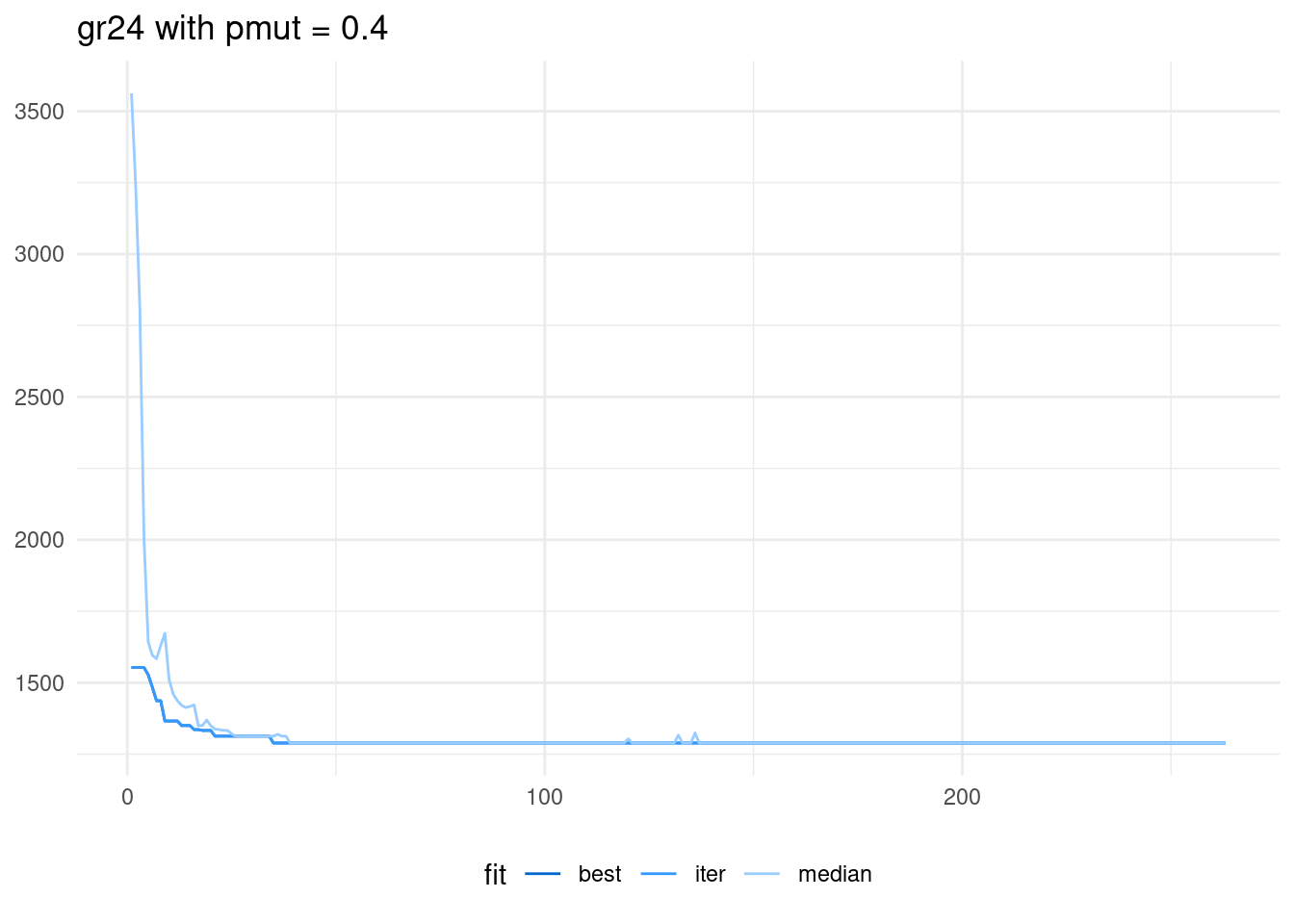
We observe that in the first iterations of the algorithm the median and the best value are similar. This means that most of the population has the same fitness function: we say that the genetic algorithm has converged. This is not desirable, as the algorithm has been stuck in a local optimum. We can add diversity to the population rising the probability of mutation to 0.8.
set.seed(11)
ga_gr24_2 <- ga_tsp(instance = gr24$D, selection = "tournament",
                  crossover = "ox", mutation = "inv", npop = 120, max_iter = 263,
                  pcross = 0.8, pmut = 0.8, elitist = TRUE, seed = TRUE)
In this case, the algorithm finds the optimal solution:
ga_gr24_2$fit## [1] 1272Let’s track the evolution of the algorithm like in the previous run:
ga_gr24_2$track |>
  pivot_longer(-step) |>
  ggplot(aes(step, value, color = name)) +
  geom_line() +
  theme_minimal() +
  theme(legend.position = "bottom") +
  labs(x = NULL, y = NULL, title = "gr24 with pmut = 0.8") +
  scale_color_manual(name = "fit", values = c("#0066CC", "#3399FF", "#99CCFF" ))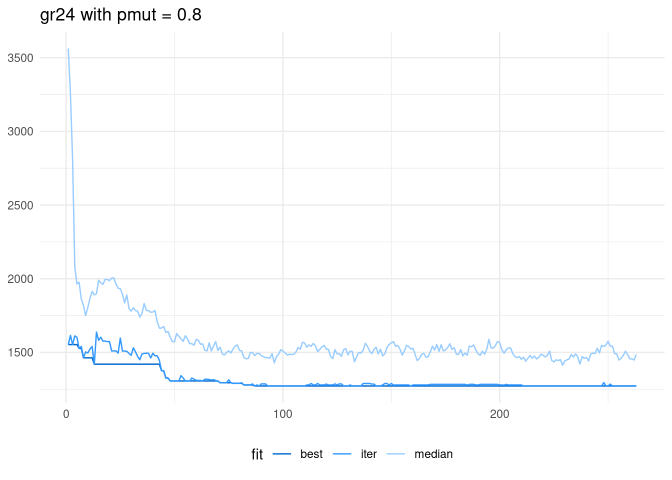
The higher probability of mutation has made the median to be way above the best solution of the iteration. This means that the population has high diversity, as it includes a wide range of values of the fitness function. In this run, the algorithm reaches the optimum in the iteration 83. Therefore, it has been more effective than tabu search for this specific instance.
Applying the algorithm to gr48
Let’s apply the algorithm to gr48, an istance from TSPLIB of n = 48 nodes. The optimal value of this instance is:
tsp_dist(gr48$D, gr48$opt.tour)## [1] 5046For this instance, I will increase the population size to 240, and establish 1350 generations to have a number of runs of the objective function similar to tabu search.
set.seed(11)
ga_gr48 <- ga_tsp(instance = gr48$D, selection = "tournament",
                  crossover = "ox", mutation = "inv", npop = 240, max_iter = 1350,
                  pcross = 0.8, pmut = 0.8, elitist = TRUE, seed = TRUE)
Here the solution is far from the optimum:
ga_gr48$fit## [1] 5293Here is the plot tracking the evolution of the algorithm.
ga_gr48$track |>
  pivot_longer(-step) |>
  ggplot(aes(step, value, color = name)) +
  geom_line() +
  theme_minimal() +
  theme(legend.position = "bottom") +
  labs(x = NULL, y = NULL, title = "gr48") +
  scale_color_manual(name = "fit", values = c("#0066CC", "#3399FF", "#99CCFF" ))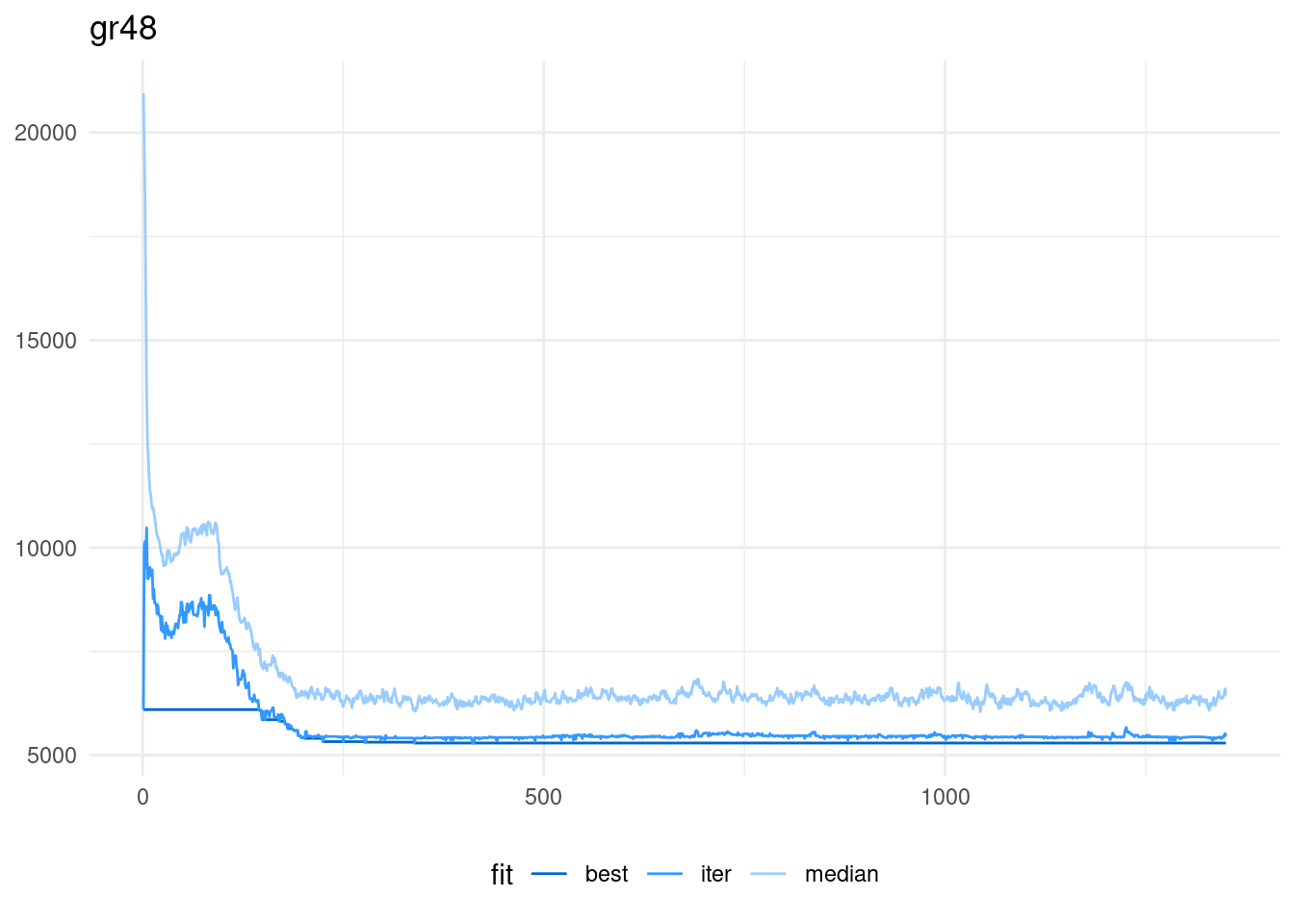
For this run of the algorithm, the high probability of mutation maintains population diversity. Again, the best value of the algorithm for this instance is obtained in the iteration 339.
Genetic Algorithms with Permutative Encoding
In this post, I have presented a genetic algorithm implementing crossover and mutation operators for permutative encoding, and I have applied it to solve two instances of the travelling salesman problem of 24 and 48 nodes. When testing the algorithms, I have set a number of evaluations of the objective function similar to the applied in testing of local search algorithms made on a previous post.
Results show that genetic algorithms can obtain results close to the optimal solution faster than simulated annealing, although in the instance of 48 nodes genetic algorithms are less effective than tabu search. Therefore, genetic algorithms can be seen as a faster, although less effective alternative to local search algorithms.
Unlike local search algorithms like simulated annealing and tabu search, genetic algorithms have a large set of parameters. This requires extensive computational experiments to tune these algorithms.
References
- 2-opt local search for the TSP. https://jmsallan.netlify.app/blog/2-opt-local-search-for-the-tsp/
- gist with code of functions: https://gist.github.com/jmsallan/1d284ccc9734cc501c2400517d798cfd
- TSPLIB http://comopt.ifi.uni-heidelberg.de/software/TSPLIB95/
Session Info
## R version 4.5.1 (2025-06-13)
## Platform: x86_64-pc-linux-gnu
## Running under: Linux Mint 21.1
##
## Matrix products: default
## BLAS:   /usr/lib/x86_64-linux-gnu/blas/libblas.so.3.10.0
## LAPACK: /usr/lib/x86_64-linux-gnu/lapack/liblapack.so.3.10.0  LAPACK version 3.10.0
##
## locale:
##  [1] LC_CTYPE=es_ES.UTF-8       LC_NUMERIC=C
##  [3] LC_TIME=es_ES.UTF-8        LC_COLLATE=es_ES.UTF-8
##  [5] LC_MONETARY=es_ES.UTF-8    LC_MESSAGES=es_ES.UTF-8
##  [7] LC_PAPER=es_ES.UTF-8       LC_NAME=C
##  [9] LC_ADDRESS=C               LC_TELEPHONE=C
## [11] LC_MEASUREMENT=es_ES.UTF-8 LC_IDENTIFICATION=C
##
## time zone: Europe/Madrid
## tzcode source: system (glibc)
##
## attached base packages:
## [1] stats     graphics  grDevices utils     datasets  methods   base
##
## other attached packages:
##  [1] lubridate_1.9.4 forcats_1.0.0   stringr_1.5.1   dplyr_1.1.4
##  [5] purrr_1.0.4     readr_2.1.5     tidyr_1.3.1     tibble_3.2.1
##  [9] ggplot2_3.5.2   tidyverse_2.0.0
##
## loaded via a namespace (and not attached):
##  [1] gtable_0.3.6      xfun_0.52         bslib_0.9.0       httr2_1.1.2
##  [5] htmlwidgets_1.6.4 devtools_2.4.5    remotes_2.5.0     gh_1.5.0
##  [9] tzdb_0.5.0        vctrs_0.6.5       tools_4.5.1       generics_0.1.3
## [13] curl_6.2.2        pkgconfig_2.0.3   lifecycle_1.0.4   farver_2.1.2
## [17] compiler_4.5.1    munsell_0.5.1     httpuv_1.6.16     htmltools_0.5.8.1
## [21] usethis_3.1.0     sass_0.4.10       yaml_2.3.10       later_1.4.2
## [25] pillar_1.10.2     jquerylib_0.1.4   urlchecker_1.0.1  ellipsis_0.3.2
## [29] cachem_1.1.0      sessioninfo_1.2.3 mime_0.13         tidyselect_1.2.1
## [33] digest_0.6.37     stringi_1.8.7     bookdown_0.43     labeling_0.4.3
## [37] fastmap_1.2.0     grid_4.5.1        colorspace_2.1-1  cli_3.6.4
## [41] magrittr_2.0.3    pkgbuild_1.4.8    withr_3.0.2       scales_1.3.0
## [45] promises_1.3.2    rappdirs_0.3.3    timechange_0.3.0  rmarkdown_2.29
## [49] httr_1.4.7        gitcreds_0.1.2    blogdown_1.21     hms_1.1.3
## [53] memoise_2.0.1     shiny_1.10.0      evaluate_1.0.3    knitr_1.50
## [57] miniUI_0.1.2      profvis_0.4.0     rlang_1.1.6       Rcpp_1.0.14
## [61] xtable_1.8-4      glue_1.8.0        pkgload_1.4.0     rstudioapi_0.17.1
## [65] jsonlite_2.0.0    R6_2.6.1          fs_1.6.6