In this post, I present an explanatory model of fuel consumption for the mtcars dataset with high explanatory power. Then, I will present an alternative model using an alternative measure of fuel consumption. This is an example of the role that a good theoretical background can do in exploratory data analysis.
The mtcars dataset presents fuel consumption and ten aspects of automobile design and performance reported on Motor Trend US in 1974. Let’s start loading the tidyverse and presenting mtcars as a tibble.
library(tidyverse)
mtcars <- mtcars |>
  mutate(model = rownames(mtcars))
mtcars <- tibble(mtcars)
mtcars
## # A tibble: 32 × 12
## mpg cyl disp hp drat wt qsec vs am gear carb model
## <dbl> <dbl> <dbl> <dbl> <dbl> <dbl> <dbl> <dbl> <dbl> <dbl> <dbl> <chr>
## 1 21 6 160 110 3.9 2.62 16.5 0 1 4 4 Mazda RX4
## 2 21 6 160 110 3.9 2.88 17.0 0 1 4 4 Mazda RX4 …
## 3 22.8 4 108 93 3.85 2.32 18.6 1 1 4 1 Datsun 710
## 4 21.4 6 258 110 3.08 3.22 19.4 1 0 3 1 Hornet 4 D…
## 5 18.7 8 360 175 3.15 3.44 17.0 0 0 3 2 Hornet Spo…
## 6 18.1 6 225 105 2.76 3.46 20.2 1 0 3 1 Valiant
## 7 14.3 8 360 245 3.21 3.57 15.8 0 0 3 4 Duster 360
## 8 24.4 4 147. 62 3.69 3.19 20 1 0 4 2 Merc 240D
## 9 22.8 4 141. 95 3.92 3.15 22.9 1 0 4 2 Merc 230
## 10 19.2 6 168. 123 3.92 3.44 18.3 1 0 4 4 Merc 280
## # ℹ 22 more rowsLet’s turn all categorical variables into factors:
mtcars <- mtcars |>
  mutate(across(c(cyl, vs:carb), as.factor))
mtcars
## # A tibble: 32 × 12
## mpg cyl disp hp drat wt qsec vs am gear carb model
## <dbl> <fct> <dbl> <dbl> <dbl> <dbl> <dbl> <fct> <fct> <fct> <fct> <chr>
## 1 21 6 160 110 3.9 2.62 16.5 0 1 4 4 Mazda RX4
## 2 21 6 160 110 3.9 2.88 17.0 0 1 4 4 Mazda RX4 …
## 3 22.8 4 108 93 3.85 2.32 18.6 1 1 4 1 Datsun 710
## 4 21.4 6 258 110 3.08 3.22 19.4 1 0 3 1 Hornet 4 D…
## 5 18.7 8 360 175 3.15 3.44 17.0 0 0 3 2 Hornet Spo…
## 6 18.1 6 225 105 2.76 3.46 20.2 1 0 3 1 Valiant
## 7 14.3 8 360 245 3.21 3.57 15.8 0 0 3 4 Duster 360
## 8 24.4 4 147. 62 3.69 3.19 20 1 0 4 2 Merc 240D
## 9 22.8 4 141. 95 3.92 3.15 22.9 1 0 4 2 Merc 230
## 10 19.2 6 168. 123 3.92 3.44 18.3 1 0 4 4 Merc 280
## # ℹ 22 more rowsLet’s use the corrr package to examine the correlations among numerical variables.
library(corrr)
mtcars |>
  select(c(mpg, disp:qsec)) |>
  correlate() |>    # correlation matrix
  rearrange() |>    # reorder values
  shave() |>        # show lower diagona
  fashion()         # present two decimals
## term mpg drat qsec hp wt disp
## 1 mpg
## 2 drat .68
## 3 qsec .42 .09
## 4 hp -.78 -.45 -.71
## 5 wt -.87 -.71 -.17 .66
## 6 disp -.85 -.71 -.43 .79 .89The highest correlation of mpg is with weight wt. It is negative, as higher weight means higher fuel consumption and therefore less miles per gallon mpg. The second variable is displacement disp, but it is highly correlated with wt, so let’s keep a parsimonious model mpg ~ wt.
mtcars |>
  ggplot(aes(wt, mpg)) +
  geom_point() +
  geom_smooth() +
  theme_minimal()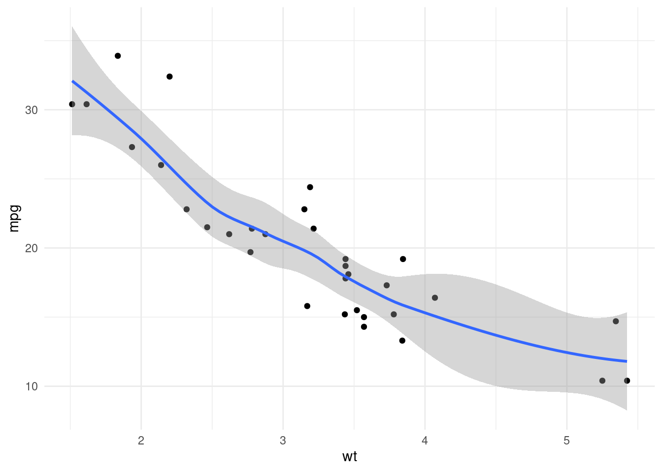
After doing a scatterplot of wt and mpg, we observe that the relationship is nonlinear. A remedy for this can be using the transmission type am variable (0 = automatic, 1 = manual).
mtcars |>
  ggplot(aes(wt, mpg, color = am)) +
  geom_point() +
  geom_smooth(method = "lm") +
  scale_color_manual(name = "transmission",
                     labels = c("automatic", "manual"),
                     values = c("red", "blue")) +
  theme_minimal() +
  theme(legend.position = "bottom")
According to this model, am moderates the relationship between wt and mpg. The slope of automatic transmission is smaller than manual, suggesting that automatic transmission reduces fuel consumption.
Let’s use the stargazer package to examine the effect of the moderating variable.
library(stargazer)
m1 <- lm(mpg ~ wt, mtcars)
m2 <- lm(mpg ~ wt*am, mtcars)
stargazer(m1, m2, type = "text")
##
## =================================================================
## Dependent variable:
## ---------------------------------------------
## mpg
## (1) (2)
## -----------------------------------------------------------------
## wt -5.344*** -3.786***
## (0.559) (0.786)
##
## am1 14.878***
## (4.264)
##
## wt:am1 -5.298***
## (1.445)
##
## Constant 37.285*** 31.416***
## (1.878) (3.020)
##
## -----------------------------------------------------------------
## Observations 32 32
## R2 0.753 0.833
## Adjusted R2 0.745 0.815
## Residual Std. Error 3.046 (df = 30) 2.591 (df = 28)
## F Statistic 91.375*** (df = 1; 30) 46.567*** (df = 3; 28)
## =================================================================
## Note: *p<0.1; **p<0.05; ***p<0.01The coefficients of variables wt and am, and of the interaction term wt:am are significant. Besides, the model with interaction term adds explanatory power to the model.
anova(m1, m2)## Analysis of Variance Table
##
## Model 1: mpg ~ wt
## Model 2: mpg ~ wt * am
## Res.Df RSS Df Sum of Sq F Pr(>F)
## 1 30 278.32
## 2 28 188.01 2 90.314 6.7253 0.004119 **
## ---
## Signif. codes: 0 '***' 0.001 '**' 0.01 '*' 0.05 '.' 0.1 ' ' 1From this model, we can conclude that fuel consumption in miles per gallon depends on car weight, and that this relationship is moderated by type of transmission.
An Alternative Measure of Fuel Consumption
While in the United States fuel consumption is measured in miles per gallon, in other parts of the word is measured in liters of fuel per 100 Km. One measure of fuel consumption is inverse of the other. Let’s calculate fuel consumption per 100 Km l100 from mpg.
mtcars <- mtcars |>
  mutate(l100 = 235.2146/mpg)
And let’s see how this measure of fuel consumption relates with weight.
mtcars |>
  ggplot(aes(wt, l100)) +
  geom_point() +
  geom_smooth() +
  theme_minimal()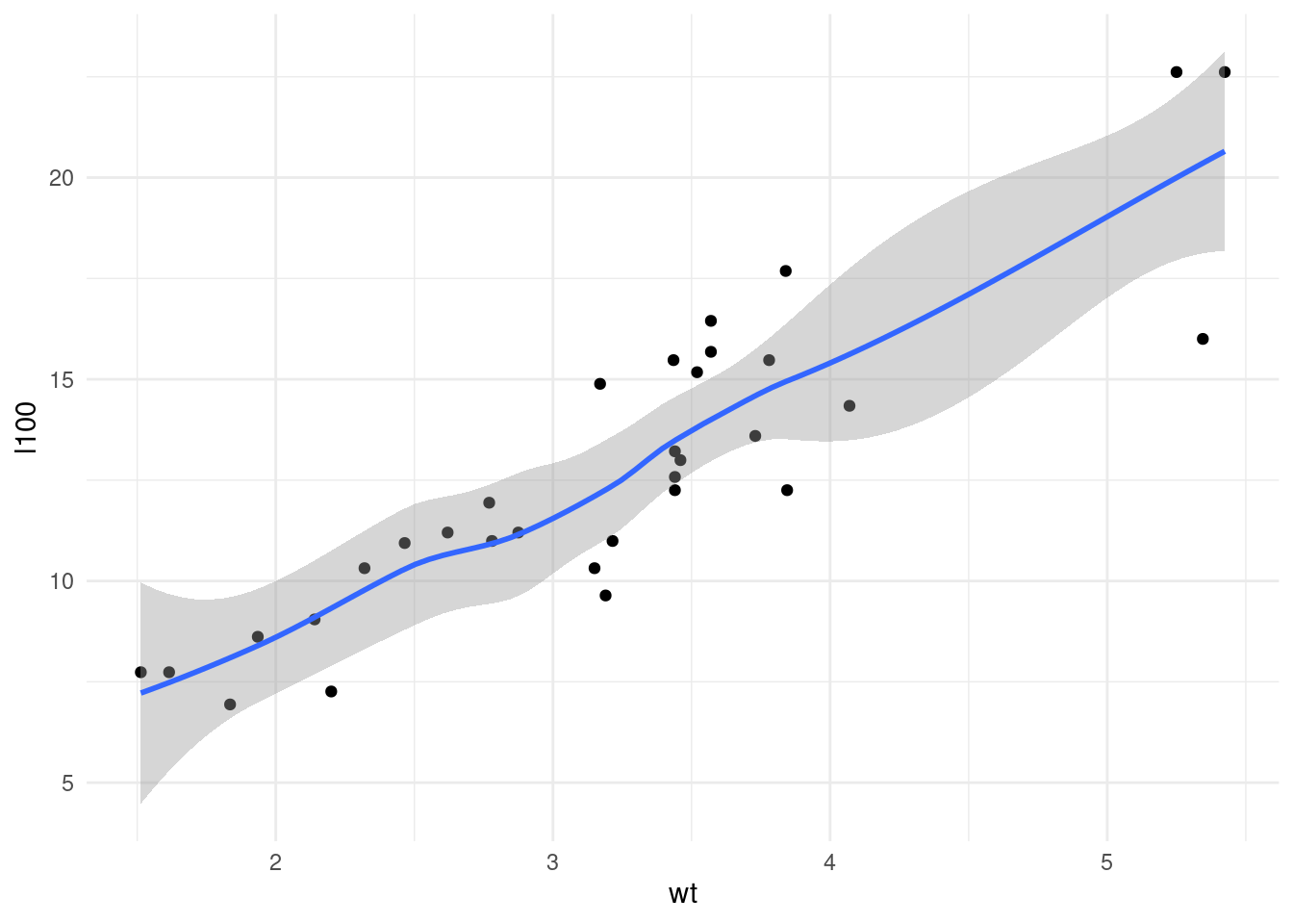
Here we observe a direct, linear relationship between wt and l100. Let’s introduce type of transmission.
mtcars |>
  ggplot(aes(wt, l100, color = am)) +
  geom_point() +
  geom_smooth(method = "lm") +
  scale_color_manual(name = "transmission",
                     labels = c("automatic", "manual"),
                     values = c("red", "blue")) +
  theme_minimal() +
  theme(legend.position = "bottom")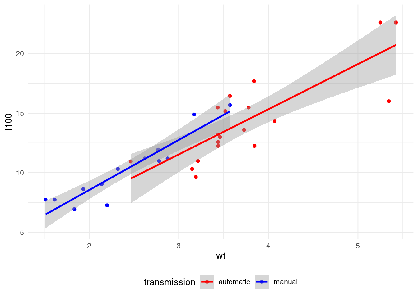
In this model, the slope of both types of transmission looks quite similar. Let’s confirm that with a regression model.
m3 <- lm(l100 ~ wt, mtcars)
m4 <- lm(l100 ~ wt*am, mtcars)
stargazer(m3, m4, type = "text")
##
## ==================================================================
## Dependent variable:
## ----------------------------------------------
## l100
## (1) (2)
## ------------------------------------------------------------------
## wt 3.514*** 3.791***
## (0.329) (0.545)
##
## am1 -0.039
## (2.959)
##
## wt:am1 0.418
## (1.003)
##
## Constant 1.451 0.165
## (1.104) (2.096)
##
## ------------------------------------------------------------------
## Observations 32 32
## R2 0.792 0.804
## Adjusted R2 0.785 0.783
## Residual Std. Error 1.791 (df = 30) 1.798 (df = 28)
## F Statistic 114.168*** (df = 1; 30) 38.365*** (df = 3; 28)
## ==================================================================
## Note: *p<0.1; **p<0.05; ***p<0.01In this model, the coefficients of am and am:wt are not significant. The analysis of variance confirms that the model with interaction terms does not add explanatory power to the model.
anova(m3, m4)## Analysis of Variance Table
##
## Model 1: l100 ~ wt
## Model 2: l100 ~ wt * am
## Res.Df RSS Df Sum of Sq F Pr(>F)
## 1 30 96.276
## 2 28 90.531 2 5.7456 0.8885 0.4225Therefore, according to this model fuel consumption in liters per kilometer depends on car weight, and we cannot appreciate any relationship between fuel consumption and type of transmission.
Which Model Is Better?
Now we have two competing models to explain fuel consumption.
- The model
m2, with formulampg ~ wt*amand adjusted R2 of 0.815. - The model
m3, with formulal100 ~ wtand adjusted R2 of 0.785.
Although m2 has a better fit than m3, I argue that the best model is m3. My choice is grounded on the plot of m2.
mtcars |>
  ggplot(aes(wt, mpg, color = am)) +
  geom_point() +
  geom_smooth(method = "lm") +
  scale_color_manual(name = "transmission",
                     labels = c("automatic", "manual"),
                     values = c("red", "blue")) +
  theme_minimal() +
  theme(legend.position = "bottom")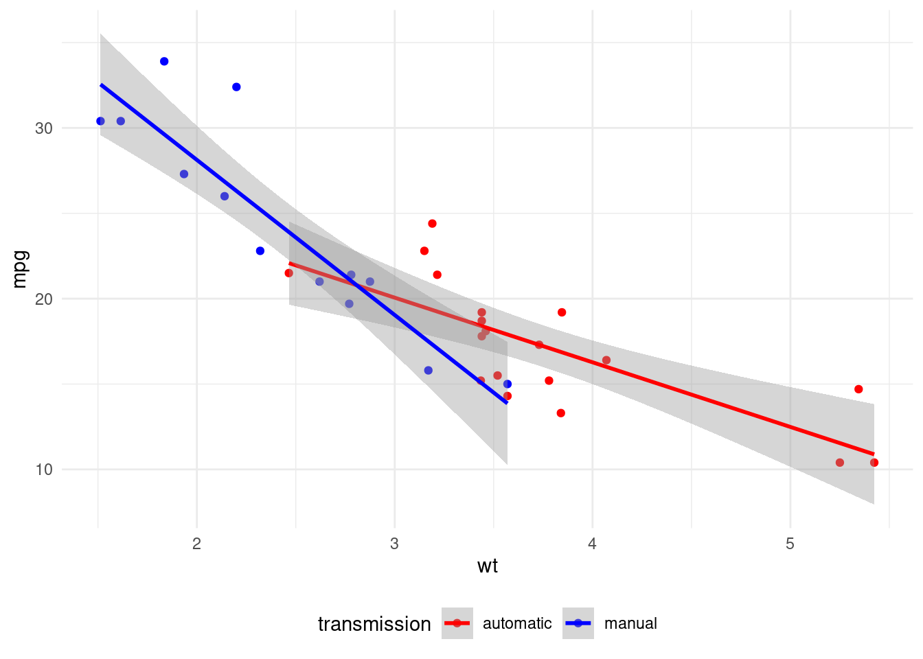
The am variable is a proxy for a variable separating light and heavy cars. While most light cars have manual transmission, heavier cars tend to have automatic transmission. This is because in 1972, American cars had automatic transmission, while European and Japanese cars tended to have manual transmission. To illustrate this, I have imputed the country of manufacturing of each model based on its name.
mtcars <- mtcars |>
  mutate(country = c(rep("J", 3),
                     rep("A", 4),
                     rep("E", 7),
                     rep("A", 3),
                     "E",
                     rep("J", 3),
                     rep("A", 4),
                     rep("E", 3),
                     "A",
                     rep("E", 3)))

mtcars |>
  ggplot(aes(wt, mpg, color = country)) +
  geom_point(size = 2) +
  theme_minimal() +
  theme(legend.position = "bottom")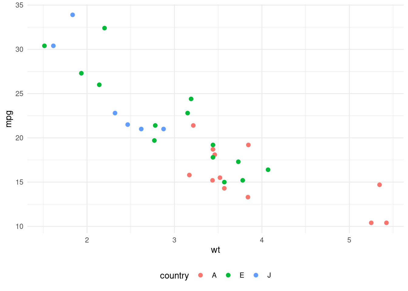
The plot shows how heavier cars (with wt > 3) tend to be American, while lighter cars are European or Japanese.
The most relevant argument favouring model m3 is that the energy requested to move a car is proportional to weight, and that fuel consumption in liters per 100 Km is a direct proxy of energy, while miles per gallon is inversely proportional to energy spent. Note that it does not have to do with units used: fuel consumption in gallons per 100 miles would be also a direct proxy of energy.
Conclusion
I argue that m3 is the model that better measures the relationship between weight and fuel consumption. Measuring fuel consumption in liters per 100 kilometers instead of miles per gallon allows using a direct proxy of energy spent to move the car, and allows finding a linear relationship between weight and fuel consumption.
Furthermore, note that plots have been a better guide than statistical models to graps the relationship between variables. This is a demonstration of the usefulness of plots in exploratory data analysis.
Session Info
## R version 4.4.3 (2025-02-28)
## Platform: x86_64-pc-linux-gnu
## Running under: Linux Mint 21.1
##
## Matrix products: default
## BLAS:   /usr/lib/x86_64-linux-gnu/blas/libblas.so.3.10.0
## LAPACK: /usr/lib/x86_64-linux-gnu/lapack/liblapack.so.3.10.0
##
## locale:
##  [1] LC_CTYPE=es_ES.UTF-8       LC_NUMERIC=C
##  [3] LC_TIME=es_ES.UTF-8        LC_COLLATE=es_ES.UTF-8
##  [5] LC_MONETARY=es_ES.UTF-8    LC_MESSAGES=es_ES.UTF-8
##  [7] LC_PAPER=es_ES.UTF-8       LC_NAME=C
##  [9] LC_ADDRESS=C               LC_TELEPHONE=C
## [11] LC_MEASUREMENT=es_ES.UTF-8 LC_IDENTIFICATION=C
##
## time zone: Europe/Madrid
## tzcode source: system (glibc)
##
## attached base packages:
## [1] stats     graphics  grDevices utils     datasets  methods   base
##
## other attached packages:
##  [1] stargazer_5.2.3 corrr_0.4.4     lubridate_1.9.4 forcats_1.0.0
##  [5] stringr_1.5.1   dplyr_1.1.4     purrr_1.0.2     readr_2.1.5
##  [9] tidyr_1.3.1     tibble_3.2.1    ggplot2_3.5.1   tidyverse_2.0.0
##
## loaded via a namespace (and not attached):
##  [1] sass_0.4.9        utf8_1.2.4        generics_0.1.3    lattice_0.22-5
##  [5] blogdown_1.19     stringi_1.8.3     hms_1.1.3         digest_0.6.35
##  [9] magrittr_2.0.3    evaluate_0.23     grid_4.4.3        timechange_0.3.0
## [13] bookdown_0.39     iterators_1.0.14  fastmap_1.1.1     Matrix_1.7-3
## [17] foreach_1.5.2     jsonlite_1.8.9    seriation_1.5.5   mgcv_1.9-1
## [21] scales_1.3.0      codetools_0.2-19  jquerylib_0.1.4   registry_0.5-1
## [25] cli_3.6.2         rlang_1.1.5       splines_4.4.3     munsell_0.5.1
## [29] withr_3.0.0       cachem_1.0.8      yaml_2.3.8        tools_4.4.3
## [33] tzdb_0.4.0        colorspace_2.1-0  ca_0.71.1         vctrs_0.6.5
## [37] TSP_1.2-4         R6_2.5.1          lifecycle_1.0.4   pkgconfig_2.0.3
## [41] pillar_1.10.1     bslib_0.7.0       gtable_0.3.5      glue_1.7.0
## [45] highr_0.10        xfun_0.43         tidyselect_1.2.1  rstudioapi_0.16.0
## [49] knitr_1.46        farver_2.1.1      nlme_3.1-168      htmltools_0.5.8.1
## [53] labeling_0.4.3    rmarkdown_2.26    compiler_4.4.3