The longley dataset was compiled by James W. Longley for his 1967 paper “An Appraisal of Least Squares Programs for the Electronic Computer.” It contains annual U.S. macroeconomic data from 1947–1962 (e.g., employment, GNP, GNP deflator, unemployment, armed forces, population, year) and was created to test the accuracy and numerical stability of regression software.
In this post I will use the dataset to examine the impact of multicollinearity on linear regression. Then, I will use an improved version of this dataset to present a non-collinear model relating macroeconomic variables.
In addition to the tidyverse, I will use corrplot to visualize correlation matrices, car to evaluate the variance inflation factor and broom for tidy extraction of data from linear models.
library(tidyverse)
library(corrplot)
library(car)
library(broom)
The original longley dataset is included in R base:
tibble(longley)## # A tibble: 16 × 7
## GNP.deflator GNP Unemployed Armed.Forces Population Year Employed
## <dbl> <dbl> <dbl> <dbl> <dbl> <int> <dbl>
## 1 83 234. 236. 159 108. 1947 60.3
## 2 88.5 259. 232. 146. 109. 1948 61.1
## 3 88.2 258. 368. 162. 110. 1949 60.2
## 4 89.5 285. 335. 165 111. 1950 61.2
## 5 96.2 329. 210. 310. 112. 1951 63.2
## 6 98.1 347. 193. 359. 113. 1952 63.6
## 7 99 365. 187 355. 115. 1953 65.0
## 8 100 363. 358. 335 116. 1954 63.8
## 9 101. 397. 290. 305. 117. 1955 66.0
## 10 105. 419. 282. 286. 119. 1956 67.9
## 11 108. 443. 294. 280. 120. 1957 68.2
## 12 111. 445. 468. 264. 122. 1958 66.5
## 13 113. 483. 381. 255. 123. 1959 68.7
## 14 114. 503. 393. 251. 125. 1960 69.6
## 15 116. 518. 481. 257. 128. 1961 69.3
## 16 117. 555. 401. 283. 130. 1962 70.6Multicollinearity
Let’s examine the correlation matrix of the dataset using corrplot().
longley |>
  cor() |>
  corrplot()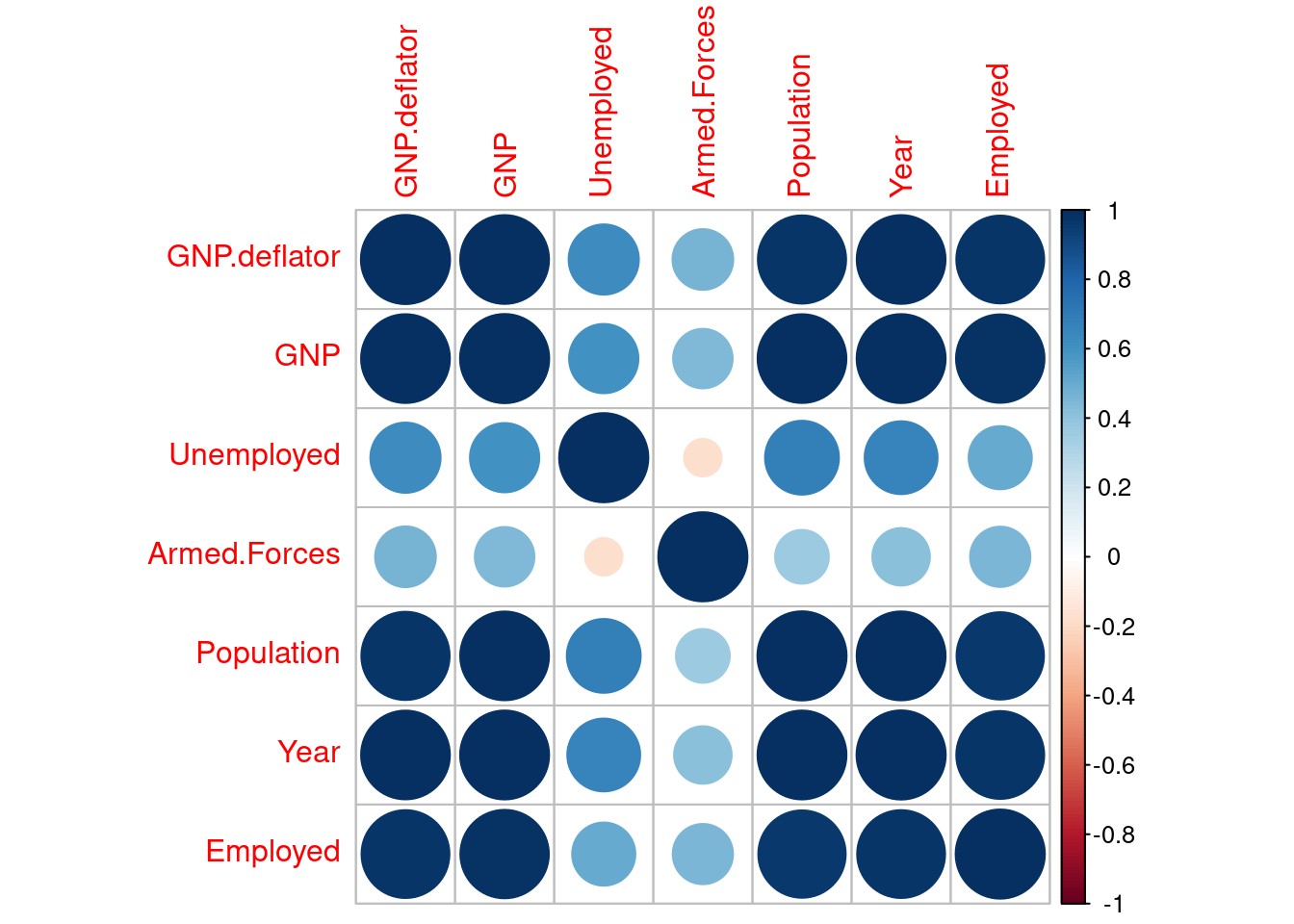
Except Unemployed and Armed.Forces, all variables are highly correlated. This can be explained by the growth of population and inflation in the US in the 1947-1962 period.
Let’s build a regression model mod01 with Employed as dependent variable including all variables.
mod01 <- lm(Employed ~ ., longley)
summary(mod01)
##
## Call:
## lm(formula = Employed ~ ., data = longley)
##
## Residuals:
## Min 1Q Median 3Q Max
## -0.41011 -0.15767 -0.02816 0.10155 0.45539
##
## Coefficients:
## Estimate Std. Error t value Pr(>|t|)
## (Intercept) -3.482e+03 8.904e+02 -3.911 0.003560 **
## GNP.deflator 1.506e-02 8.492e-02 0.177 0.863141
## GNP -3.582e-02 3.349e-02 -1.070 0.312681
## Unemployed -2.020e-02 4.884e-03 -4.136 0.002535 **
## Armed.Forces -1.033e-02 2.143e-03 -4.822 0.000944 ***
## Population -5.110e-02 2.261e-01 -0.226 0.826212
## Year 1.829e+00 4.555e-01 4.016 0.003037 **
## ---
## Signif. codes: 0 '***' 0.001 '**' 0.01 '*' 0.05 '.' 0.1 ' ' 1
##
## Residual standard error: 0.3049 on 9 degrees of freedom
## Multiple R-squared: 0.9955, Adjusted R-squared: 0.9925
## F-statistic: 330.3 on 6 and 9 DF, p-value: 4.984e-10In this model, Year, Unemployed and Armed.Forces show a significant relationship with Employed. Although GNP, GNP.deflator and Population are highly correlated with the dependent variable, the regression coefficients are not significant. This is an example of multicollinearity: when dependent variables are highly correlated, the standard errors of the coefficients are inflated and then they can appear as non significant. Standard errors appear in the Std. Error column of the model summary.
A diagnostic of multicollinearity is the variance inflation factor (VIF). The VIF of a variable is obtained regressing the variable on the rest of dependent variables. Values of VIF above 10 are an indicator of high multicollinearity.
We can obtain VIFs with the car::vif() function.
vif(mod01)## GNP.deflator GNP Unemployed Armed.Forces Population Year
## 135.53244 1788.51348 33.61889 3.58893 399.15102 758.98060In mod01 all variables except Armed.Forces show high multicollinearity.
To show how introducing high correlated independent variables affects results, let’s build a regression of Employed on GNP only. GNP had a non significant coefficient in the previous model.
mod02 <- lm(Employed ~ GNP, longley)
summary(mod02)
##
## Call:
## lm(formula = Employed ~ GNP, data = longley)
##
## Residuals:
## Min 1Q Median 3Q Max
## -0.77958 -0.55440 -0.00944 0.34361 1.44594
##
## Coefficients:
## Estimate Std. Error t value Pr(>|t|)
## (Intercept) 51.843590 0.681372 76.09 < 2e-16 ***
## GNP 0.034752 0.001706 20.37 8.36e-12 ***
## ---
## Signif. codes: 0 '***' 0.001 '**' 0.01 '*' 0.05 '.' 0.1 ' ' 1
##
## Residual standard error: 0.6566 on 14 degrees of freedom
## Multiple R-squared: 0.9674, Adjusted R-squared: 0.965
## F-statistic: 415.1 on 1 and 14 DF, p-value: 8.363e-12While in mod01 the coefficient of GNP was non significant, in mod02 is highly significant. The standard error of the coefficient of GNP was of 0.03 in mod01, and of 0.002 in mod02: this error was 19 times higher in mod01 than in mod02.
The value of Population is of people of age greter or equal than fourteen years. Then, we may think that the total Population is larger than the sum of Employed, Unemployed or enroled in Armed.Forces.
longley |>
  select(Year, Unemployed, Employed, Armed.Forces, Population) |>
  pivot_longer(-Year) |>
  ggplot(aes(Year, value, color = name)) +
  geom_line(linewidth = 1) +
  scale_color_manual(values = c("#990000", "#FF8000", "#0080FF", "#CCCC00")) +
  theme_minimal(base_size = 12) +
  theme(legend.position = "bottom") +
  labs(x = NULL, y = NULL, title = "Evolution of population variables longley")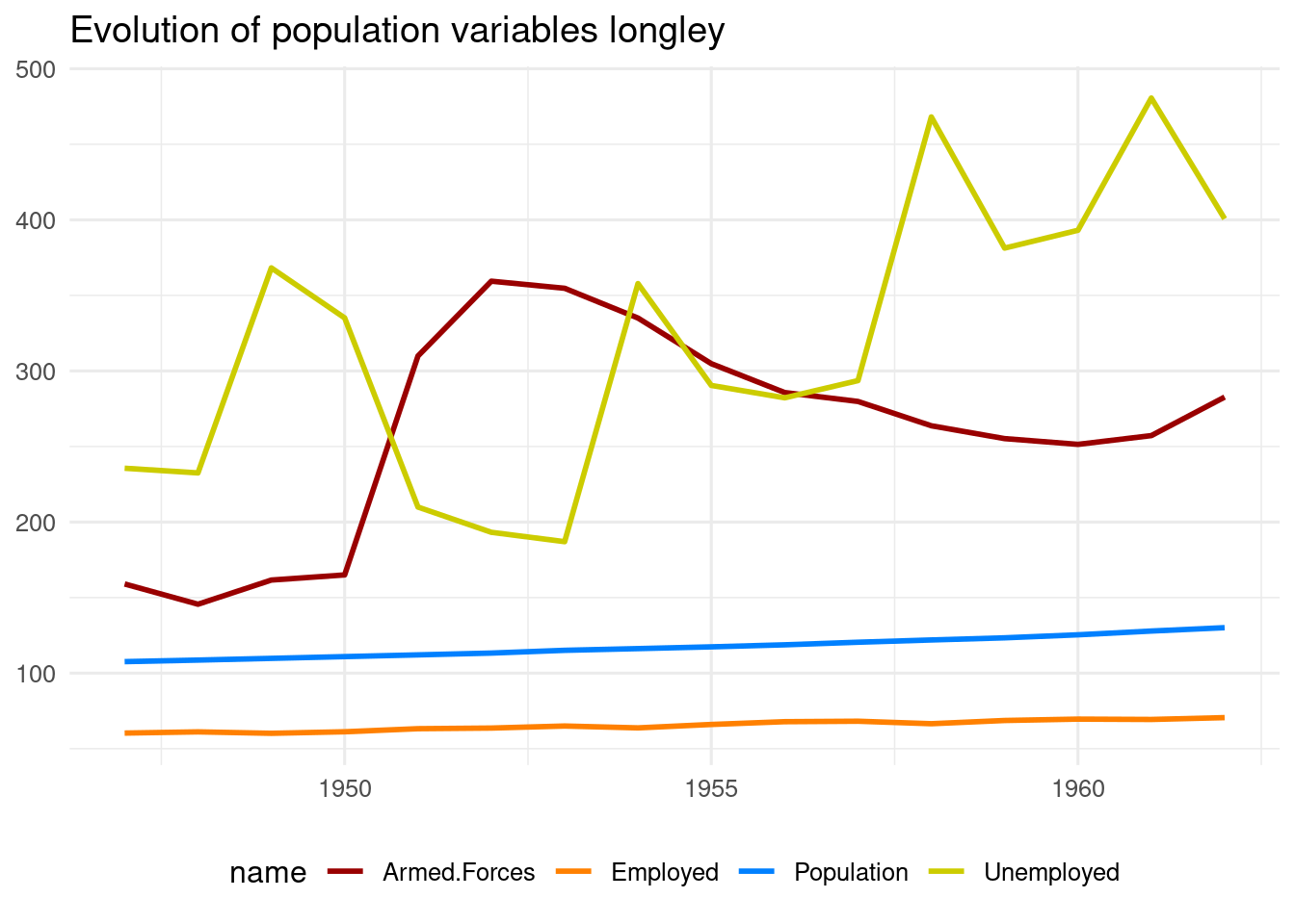
The representation of the variables shows that the values of population are inconsistent, as the number of people in the Armed Forces and unemployed are much larger than total population.
A Better longley Dataset: longley2
In the RXshrink package, we can find a longley2 dataset. It includes data from the Employment and Training Report of the President, 1976 compiled by Art Hoerl, from the University of Delaware. This data frame contains some different (“corrected”) numerical values from those used by Longley (1967) and the added years of 1963-1975.
tibble(longley2)## # A tibble: 29 × 7
## GNP.deflator Unemployed Armed.Forces Population Year Employed GNP
## <dbl> <int> <int> <int> <int> <int> <dbl>
## 1 83.6 2311 1591 103418 1947 59805 233.
## 2 89 2276 1459 104527 1948 60632 259.
## 3 88.1 3637 1617 105611 1949 59640 258
## 4 89.9 3288 1650 106645 1950 60645 286.
## 5 95.9 2055 3100 107721 1951 62673 330.
## 6 97.2 1883 3592 108823 1952 63135 347.
## 7 98.6 1834 3545 110601 1953 64508 366.
## 8 100 3532 3350 111671 1954 63288 366.
## 9 102. 2852 3049 112732 1955 65541 399.
## 10 105. 2750 2857 113811 1956 67298 421.
## # ℹ 19 more rowsFor this dataset, quantities make sense. The difference between total population and the other three variables are people not willing to work.
longley2 |>
  select(Year, Unemployed, Employed, Armed.Forces, Population) |>
  pivot_longer(-Year) |>
  ggplot(aes(Year, value, color = name)) +
  geom_line(linewidth = 1) +
  scale_color_manual(values = c("#990000", "#CC0000", "#0080FF", "#FF3333")) +
  theme_minimal() +
  theme(legend.position = "bottom") +
  labs(x = NULL, y = NULL, title = "Evolution of population variables longley2")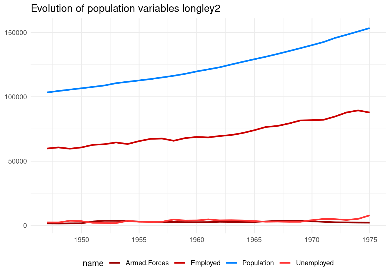
Macroeconomic Variables
longley2 allows obtaining variables more related with macroeconomic theory.
| Variable | Description |
|---|---|
year |
Year of the observation. |
deflacted_gnp_growth |
Growth of the deflacted GNP. |
activity_rate |
Fraction of the population willing to work (active). |
unemployment_rate |
Fraction of active population without employment. |
inflation |
Yearly inflation obtained from the GNP deflactor. |
longley2_mod <- longley2 |>
  mutate(deflacted_gnp = GNP*100/GNP.deflator,
         activity_rate = (Unemployed + Employed + Armed.Forces)*100/Population,
         unemployment_rate = Unemployed*100/(Unemployed + Employed + Armed.Forces),
         inflation = (GNP.deflator - lag(GNP.deflator))*100/lag(GNP.deflator),
         deflacted_gnp_growth = (deflacted_gnp - lag(deflacted_gnp))*100/lag(deflacted_gnp)) |>
  filter(!is.na(inflation)) |>
  rename(year = Year) |>
  select(year, deflacted_gnp_growth, activity_rate, unemployment_rate, inflation)
All these variables are listed in longley2_mod.
tibble(longley2_mod)## # A tibble: 28 × 5
## year deflacted_gnp_growth activity_rate unemployment_rate inflation
## <int> <dbl> <dbl> <dbl> <dbl>
## 1 1948 4.54 61.6 3.54 6.46
## 2 1949 0.593 61.4 5.60 -1.01
## 3 1950 8.71 61.5 5.01 2.04
## 4 1951 8.16 63.0 3.03 6.67
## 5 1952 3.74 63.0 2.74 1.36
## 6 1953 3.95 63.2 2.62 1.44
## 7 1954 -1.35 62.8 5.03 1.42
## 8 1955 6.77 63.4 3.99 2.10
## 9 1956 2.06 64.1 3.77 3.23
## 10 1957 1.87 63.6 3.90 3.32
## # ℹ 18 more rowsAs the new variables refer either to yearly change or are indices independent of total population the correlations among them are lower.
longley2_mod |>
  cor() |>
  corrplot()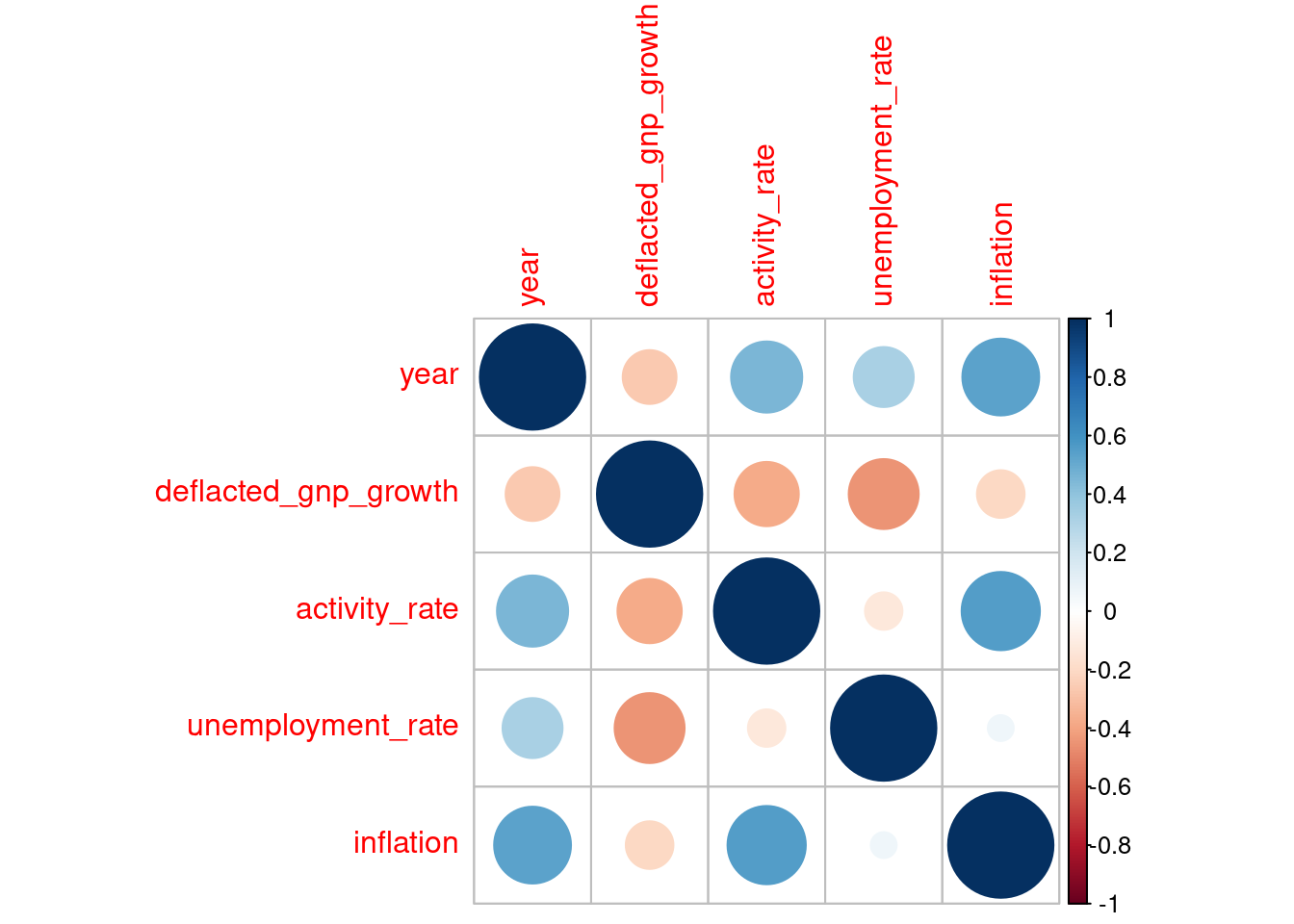
Here is the temporal evolution of the variables. For years 1974 and 1975 we can see the effect on unemployment and inflation of the oil shock crisis which started in 1973 (see the dashed red line).
labels <- c("deflacted_gnp_growth" = "gnp",
            "activity_rate" = "activity",
            "unemployment_rate" = "unemp.",
            "inflation" = "inflation")

longley2_mod |>
  pivot_longer(-year) |>
  ggplot(aes(year, value)) +
  geom_line(linewidth = 1) +
  geom_vline(xintercept = 1973, lty = "dashed", color = "red") +
  facet_grid(name ~ ., scale = "free",
             labeller = as_labeller(labels)) +
  theme_minimal() +
  labs(x = NULL, y = NULL, title = "Evolution of Macroeconomic Variables")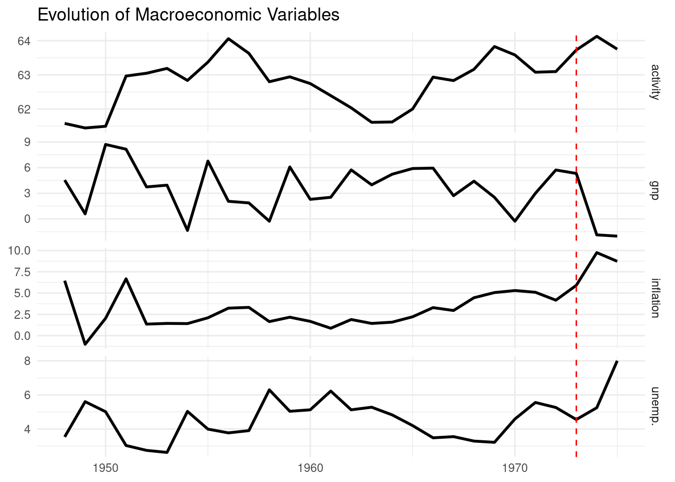
In this plot I have represented the values of unemployment and inflation for each year.
longley2_mod |>
  ggplot(aes(unemployment_rate, inflation)) +
  geom_label(aes(label = year)) +
  geom_smooth(data = longley2_mod |> filter(year <= 1973),
              aes(unemployment_rate, inflation),
              method = "lm") +
  theme_minimal() +
  labs(x = "unemployment", y = "inflation", title = "Relationship Unemployment and Inflation")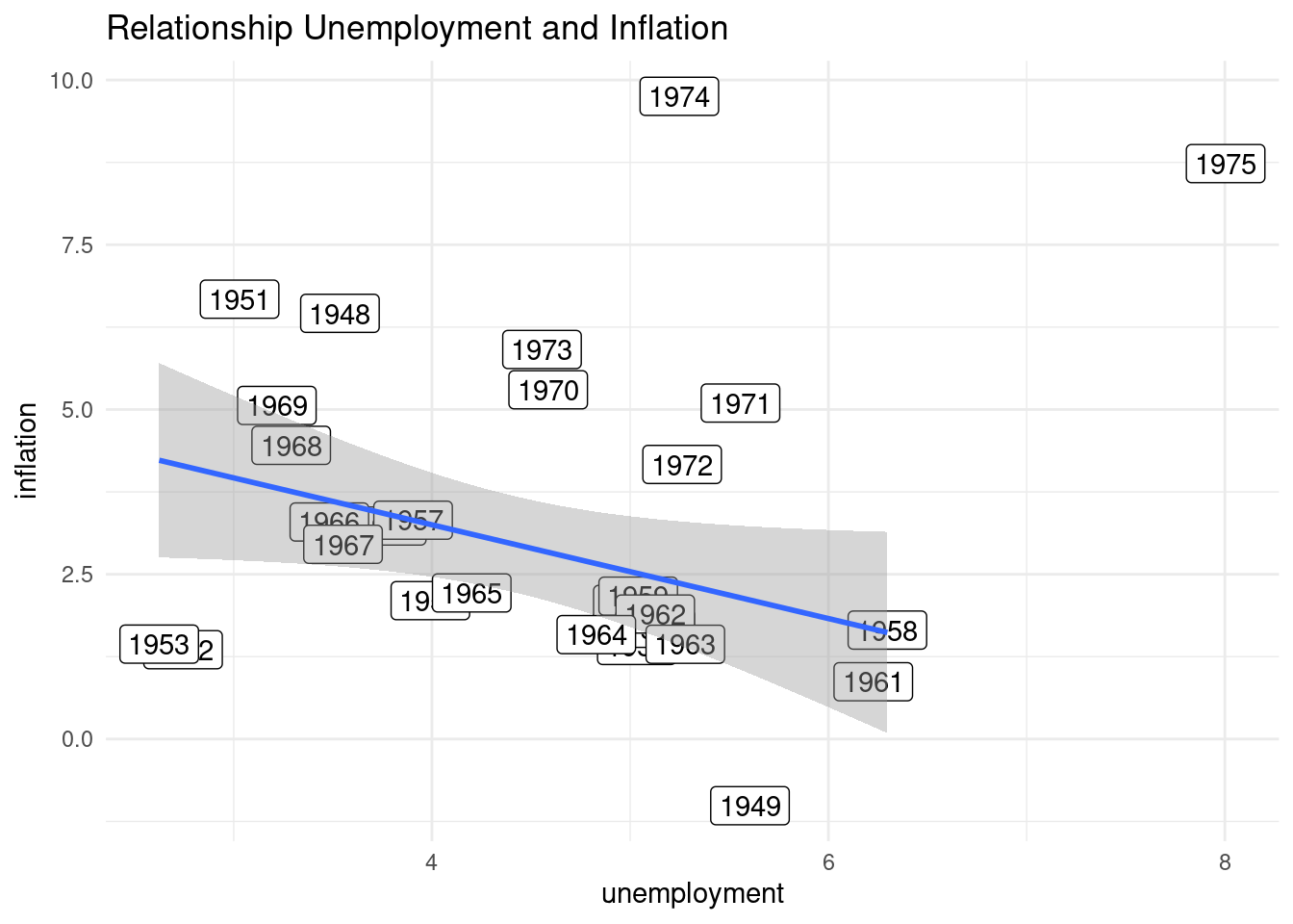
We can see how 1974 and 1975 have abormal high values of inflation and unemployment, as a result of the supply shock of the oil crisis. In the other years we can see how these variables have a negative relationship, associated to shifts of demand.
A Regression Model with longley2
Let’s build a regression model mod03, relating unemployment with GNP growth and inflation.
mod03 <- lm(unemployment_rate ~ deflacted_gnp_growth + inflation, longley2_mod)
summary(mod03)
##
## Call:
## lm(formula = unemployment_rate ~ deflacted_gnp_growth + inflation,
## data = longley2_mod)
##
## Residuals:
## Min 1Q Median 3Q Max
## -1.88371 -0.82896 0.05024 0.92969 2.47904
##
## Coefficients:
## Estimate Std. Error t value Pr(>|t|)
## (Intercept) 5.27589 0.49372 10.686 8.27e-11 ***
## deflacted_gnp_growth -0.18907 0.07740 -2.443 0.022 *
## inflation -0.01514 0.09009 -0.168 0.868
## ---
## Signif. codes: 0 '***' 0.001 '**' 0.01 '*' 0.05 '.' 0.1 ' ' 1
##
## Residual standard error: 1.136 on 25 degrees of freedom
## Multiple R-squared: 0.1957, Adjusted R-squared: 0.1314
## F-statistic: 3.041 on 2 and 25 DF, p-value: 0.06572In this model, that unemployment is negatively related with GNP growth. This means that when GNP is contracting, unemployment arises. Unemployment has a weak relationship with inflation. Although the coefficient is negative, it is not significant.
Let’s evaluate multicollinearity computing VIF.
vif(mod03)## deflacted_gnp_growth inflation
## 1.043836 1.043836All VIF values are close to one, so we can discard multicollinearity.
Finally, let’s plot standardized residuals against fitted values. I have labelled the observations with absolute value of standardized residuals larger than two. I have used broom::augment() to get the residuals .std.resid and fitted values .fitted.
resid_data <- augment(mod03) |>
  bind_cols(longley2_mod |> select(year))

resid_data |>
  ggplot(aes(.fitted, .std.resid)) +
  geom_point() +
  geom_smooth(se = FALSE, color = "red") +
  theme_minimal() +
  geom_label(data = resid_data |> filter(abs(.std.resid) >2),
             aes(x = .fitted, y = .std.resid, label = year)) +
labs(x = "fitted values", y = "std residuals", title = "Fitted values vs residuals") 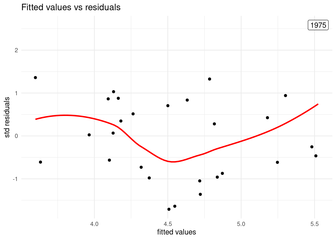
The plot of residuals shows that the variance is stable along fitted values. The only abnormal value is the observation of 1975, heavily affected by the oil crisis.
To test for normality of residuals, I have built a quantile-quantile plot (QQ-plot). This can be accomplished with stat_qq() and stat_qq_line() setting aes(sample = .std.resid).
resid_data |>
  ggplot(aes(sample = .std.resid)) +
  stat_qq(size = 1) +
  stat_qq_line() +
  theme_minimal() +
  labs(x = NULL, y = NULL, title = "QQ-plot of residuals")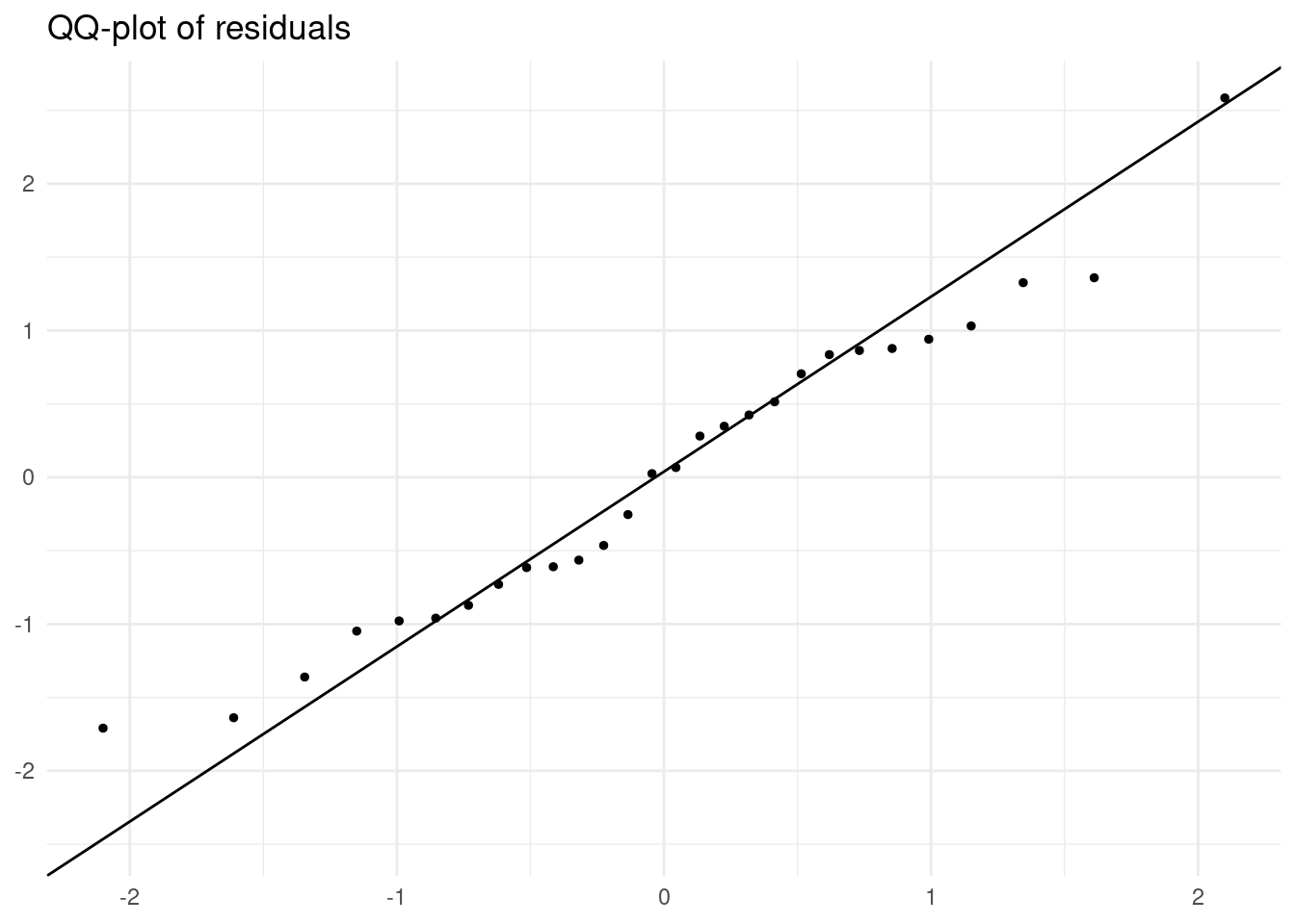
As most values are along the line, it si reaasonable to suppose that the residuals follow a normal distribution.
The Two Longley Datasets
The longley dataset has been used to show the impact of having highly correlated dependent variables in linear regression. Beyond that, this dataset is quite short (only 16 observations) and has significant errors in the values related to population to be usable beyond showing the problems of multicollinearity.
The longley2 has a longer series of data and the values of population are corrected. Most variables are also highly correlated, but this dataset has allowed me to define ratios of components of population and a metric of inflation.
These variables have lower values of correlation, and allow to illustrate some basic relationship between economic growth, unemployment and inflation. While results show a negative relationship between economic growth and unemployment, the relationship between growth and employment is too weak to be statistically significant.
References
- Longley, J. W. (1967). An appraisal of least squares programs for the electronic computer from the point of view of the user. Journal of the American Statistical association, 62(319), 819-841.
- Art Hoerl’s update of the infamous Longley(1967) benchmark dataset. https://search.r-project.org/CRAN/refmans/RXshrink/html/longley2.html.
Session Info
## R version 4.5.2 (2025-10-31)
## Platform: x86_64-pc-linux-gnu
## Running under: Linux Mint 21.1
##
## Matrix products: default
## BLAS:   /usr/lib/x86_64-linux-gnu/blas/libblas.so.3.10.0
## LAPACK: /usr/lib/x86_64-linux-gnu/lapack/liblapack.so.3.10.0  LAPACK version 3.10.0
##
## locale:
##  [1] LC_CTYPE=es_ES.UTF-8       LC_NUMERIC=C
##  [3] LC_TIME=es_ES.UTF-8        LC_COLLATE=es_ES.UTF-8
##  [5] LC_MONETARY=es_ES.UTF-8    LC_MESSAGES=es_ES.UTF-8
##  [7] LC_PAPER=es_ES.UTF-8       LC_NAME=C
##  [9] LC_ADDRESS=C               LC_TELEPHONE=C
## [11] LC_MEASUREMENT=es_ES.UTF-8 LC_IDENTIFICATION=C
##
## time zone: Europe/Madrid
## tzcode source: system (glibc)
##
## attached base packages:
## [1] stats     graphics  grDevices utils     datasets  methods   base
##
## other attached packages:
##  [1] broom_1.0.10    car_3.1-3       carData_3.0-5   corrplot_0.95
##  [5] lubridate_1.9.4 forcats_1.0.1   stringr_1.6.0   dplyr_1.1.4
##  [9] purrr_1.2.0     readr_2.1.5     tidyr_1.3.1     tibble_3.3.0
## [13] ggplot2_4.0.0   tidyverse_2.0.0
##
## loaded via a namespace (and not attached):
##  [1] sass_0.4.10        generics_0.1.3     lattice_0.22-5     blogdown_1.21
##  [5] stringi_1.8.7      hms_1.1.4          digest_0.6.37      magrittr_2.0.4
##  [9] evaluate_1.0.3     grid_4.5.2         timechange_0.3.0   RColorBrewer_1.1-3
## [13] bookdown_0.43      fastmap_1.2.0      Matrix_1.7-4       jsonlite_2.0.0
## [17] backports_1.5.0    Formula_1.2-5      mgcv_1.9-1         scales_1.4.0
## [21] jquerylib_0.1.4    abind_1.4-8        cli_3.6.4          rlang_1.1.6
## [25] splines_4.5.2      withr_3.0.2        cachem_1.1.0       yaml_2.3.10
## [29] tools_4.5.2        tzdb_0.5.0         vctrs_0.6.5        R6_2.6.1
## [33] lifecycle_1.0.4    pkgconfig_2.0.3    pillar_1.11.1      bslib_0.9.0
## [37] gtable_0.3.6       glue_1.8.0         xfun_0.52          tidyselect_1.2.1
## [41] rstudioapi_0.17.1  knitr_1.50         farver_2.1.2       nlme_3.1-168
## [45] htmltools_0.5.8.1  rmarkdown_2.29     labeling_0.4.3     compiler_4.5.2
## [49] S7_0.2.0