In this post, I will present the possiblities of some of the family of map_*() functions from the tidyverse purrr package. The purrr package is included in the core tydiverse packages, so we can load it doing:
library(tidyverse)I will apply these functions to present empirical evidence of the central limit theorem.
The central limit theorem states that if we collect a large enough sample of \(n\) indenpendent obaservations of a random variable with population mean \(\mu\) and stardard deviation \(\sigma\), the sample mean follows a distribution:
\[ \bar{x} \sim N\left( \mu, \sigma/\sqrt{n} \right) \]
The value \(\sigma/\sqrt{n}\) is called standard error.
To examine this theorem empirically, we need to generate several samples of the random variable and obtain the sample mean \(\bar{x}\) from each sample. Once obtained the set of sample values of \(\bar{x}\), we need to examine the mean, standard deviation and distribution. As the central limit theorem works with any distribution I will test it with:
- A normal distribution.
- A continuous uniform distribution.
Normal Distribution
The purrr::map() function iterates a function along the components of a list or vector and returns a list as output. It is largely an equivalent of the R base lapply() function.
Let’s use map() to create 1,000 samples of 2,000 observations each from a normal distribution of mean zero and three different values of standard deviation sd.
set.seed(11)
sd_05 <- map(1:1000, ~ rnorm(2000, mean = 0, sd = 0.5))
sd_10 <- map(1:1000, ~ rnorm(2000, mean = 0, sd = 1))
sd_20 <- map(1:1000, ~ rnorm(2000, mean = 0, sd = 2))

norm <- list(sd_05 = sd_05, sd_10 = sd_10, sd_20 = sd_20)
We can check the number of elements of each component of norm applying lenght() with purrr::map_int().
map_int(norm, length)## sd_05 sd_10 sd_20
## 1000 1000 1000The output of this function is a vector of integer values of sample mean \(\bar{x}\). This output inherits the names of the original norm list.
Let’s calculate \(\bar{x}\) of each of the samples of norm. The result will be a list of three components, each of them being a vector with the mean of each of the 1,000 samples. These vectors are obtained with the purrr::map_dbl() function. This function returns always a vector of double (floating point numeric) values.
mean_norm <- map(norm, ~ map_dbl(. , mean))Now we have 1,000 values of the sample mean of normal distributions with different values of standard deviation. We can obtain an estimation of the mean of the sample mean for each distribution doing:
map_dbl(mean_norm, mean)## sd_05 sd_10 sd_20
## 7.675551e-05 6.811647e-04 1.890621e-03We observe that the mean of \(\bar{x}\) is very close to \(\mu\) for the three sets of samples. Let’s look at the standard deviation:
map_dbl(mean_norm, ~ sd(.))## sd_05 sd_10 sd_20
## 0.01088386 0.02154560 0.04467244The standard deviation of \(\bar{x}\) increases as the standard deviation of the distribution increases. Let’s compare the values obtained above with the population standard error.
c(0.5, 1, 2)/sqrt(2000)## [1] 0.01118034 0.02236068 0.04472136The sample values of standard error are close to the population values.
Let’s now plot the distribution of the sample mean. To do so, I will wrap all the values of mean_norm in a single tibble with columns value and name equal to means of each sample and the name of the list of samples, respectively. We obtain that with purrr::map2_dfr():
- Being a
map2*()function,map2_dfr()takes two lists of vectors as arguments, passed as.xand.yin the formula. - Being a
map*_dfr()function,map2_dfr()binds the result into a tibble by row.
norm_table <- map2_dfr(mean_norm, names(mean_norm), ~ tibble(value = .x, name = .y))
norm_table
## # A tibble: 3,000 × 2
## value name
## <dbl> <chr>
## 1 0.00155 sd_05
## 2 0.0108 sd_05
## 3 0.0119 sd_05
## 4 -0.000436 sd_05
## 5 0.00463 sd_05
## 6 -0.00281 sd_05
## 7 0.00336 sd_05
## 8 -0.0106 sd_05
## 9 0.0114 sd_05
## 10 -0.0168 sd_05
## # ℹ 2,990 more rowsLet’s draw an histogram for each distribution:
norm_table |>
  ggplot(aes(value)) +
  geom_histogram(bins = 30) +
  facet_grid(. ~ name) +
  theme_linedraw() +
  labs(title = "Normal distribution", x = NULL, y = NULL)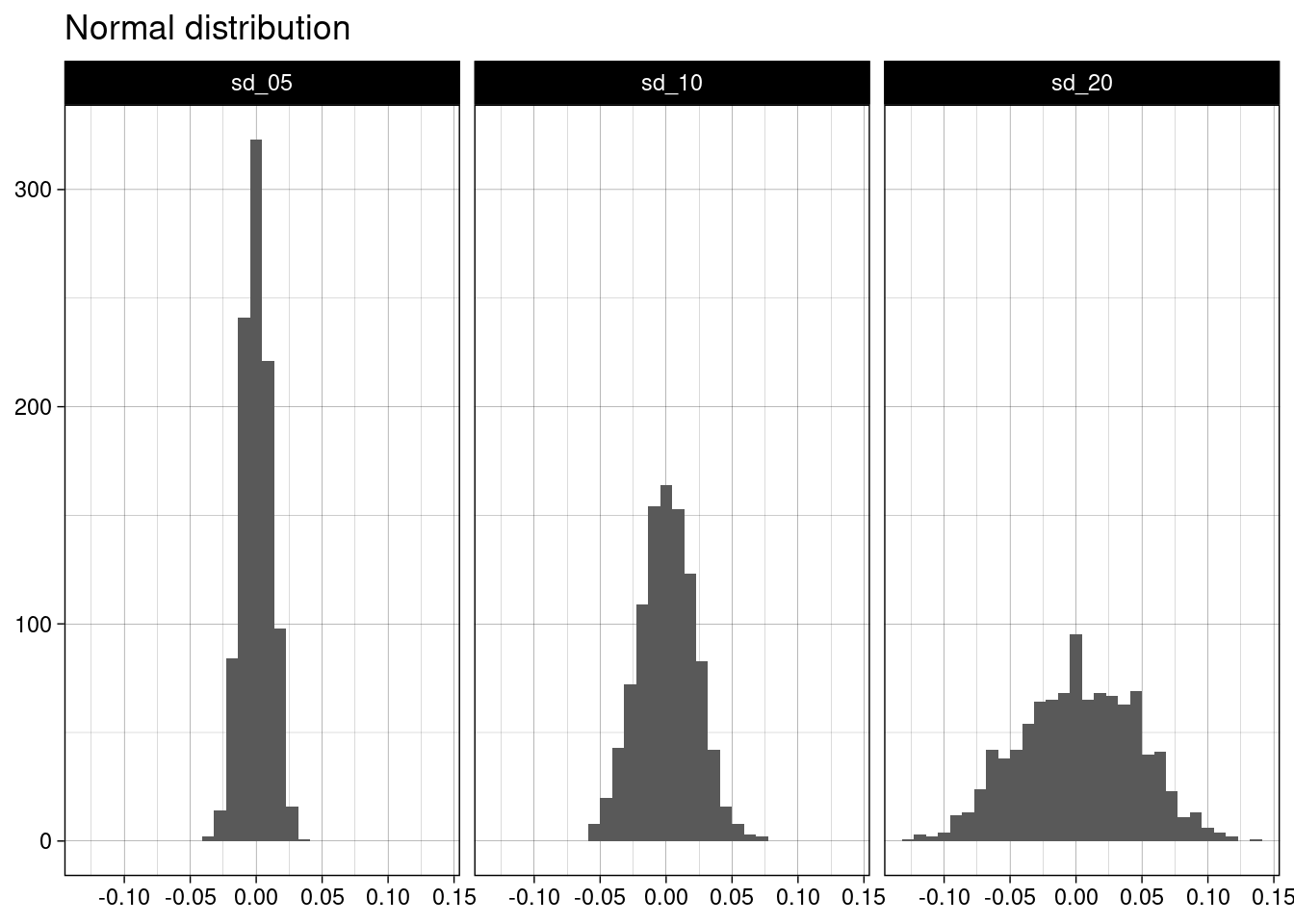
Each of the samples of \(\bar{x}\) follows a normal distribution centered in \(\mu\) and standard deviation equal to the standard error. This is what the central limit theorem states, so we have tested it empirically.
I can provide additional graphical evidence of the normality of sample mean with a quantile-quantile (Q-Q) plot, obtained with stat_qq() and stat_qq_line() from ggplot.
norm_table |>
  ggplot(aes(sample = value)) +
  stat_qq() +
  stat_qq_line(color = "red") +
  facet_grid(. ~ name) +
  theme_linedraw() +
  labs(title = "Normal distribution", x = NULL, y = NULL)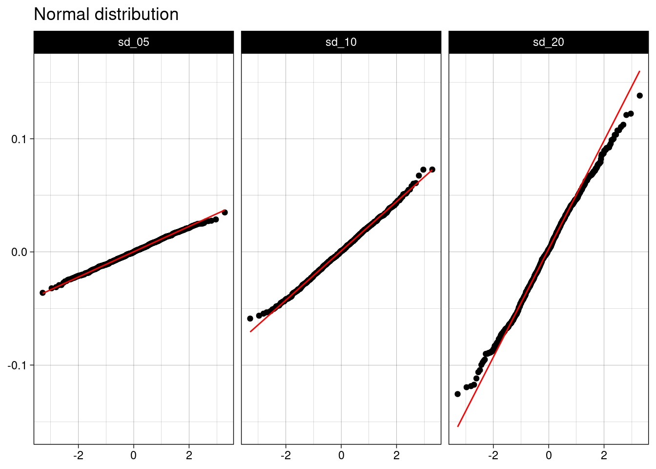
All points are aligned alog the red line, meaning that the sample follows a normal distribution.
Continuous Uniform Distribution
For the continuous uniform distribution, I will replicate the workflow of the normal distribution obtaining three samples of growing standard deviation. For a continuous distribution, the larger the difference betweem maximum and minimum, the larger the standard deviation of the distribution.
set.seed(55)
unif_01 <- map(1:1000, ~ runif(2000, min = -1, max = 1))
unif_02 <- map(1:1000, ~ runif(2000, min = -2, max = 2))
unif_04 <- map(1:1000, ~ runif(2000, min = -4, max = 4))

unif <- list(unif_01 = unif_01, unif_02 = unif_02, unif_04 = unif_04)
Like with normal distributions, let’s compute the sample means \(\bar{x}\) for each sample.
mean_unif <- map(unif, ~ map_dbl(. , mean))When computing the mean and standard deviation of the samples of \(\bar{x}\), we observe that mean is close to zero and that standard error grows:
map_dbl(mean_unif, mean)## unif_01 unif_02 unif_04
## -0.0002933102 -0.0010177496 -0.0009016651map_dbl(mean_unif, ~ sd(.))## unif_01 unif_02 unif_04
## 0.01292212 0.02627455 0.05129232Values of standard errors are close to the population values.
c(2, 4, 8)/sqrt(12*2000)## [1] 0.01290994 0.02581989 0.05163978Let’s create the tibble to plot histograms of \(\bar{x}\).
unif_table <- map2_dfr(mean_unif, names(mean_unif), ~ tibble(value = .x, name = .y))
unif_table
## # A tibble: 3,000 × 2
## value name
## <dbl> <chr>
## 1 -0.00411 unif_01
## 2 0.00394 unif_01
## 3 0.00867 unif_01
## 4 -0.0155 unif_01
## 5 -0.0350 unif_01
## 6 -0.0151 unif_01
## 7 0.00923 unif_01
## 8 -0.00413 unif_01
## 9 -0.00681 unif_01
## 10 0.00407 unif_01
## # ℹ 2,990 more rowsThese histograms show that sample means of uniform distributions are normally distributed.
unif_table |>
  ggplot(aes(value)) +
  geom_histogram(bins = 30) +
  facet_grid(. ~ name) +
  theme_linedraw() +
  labs(title = "Uniform distribution", x = NULL, y = NULL)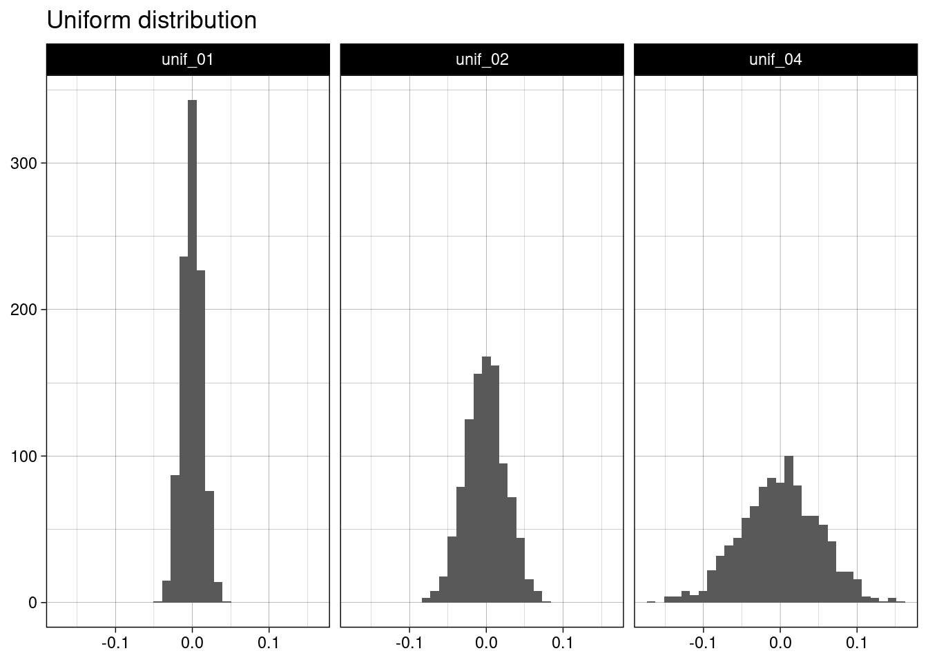
As in the previous example, I am presenting Q-Q plots to provide additional evidence of the normality of the sample mean.
unif_table |>
  ggplot(aes(sample = value)) +
  stat_qq() +
  stat_qq_line(color = "red") +
  facet_grid(. ~ name) +
  theme_linedraw() +
  labs(title = "Uniform distribution", x = NULL, y = NULL)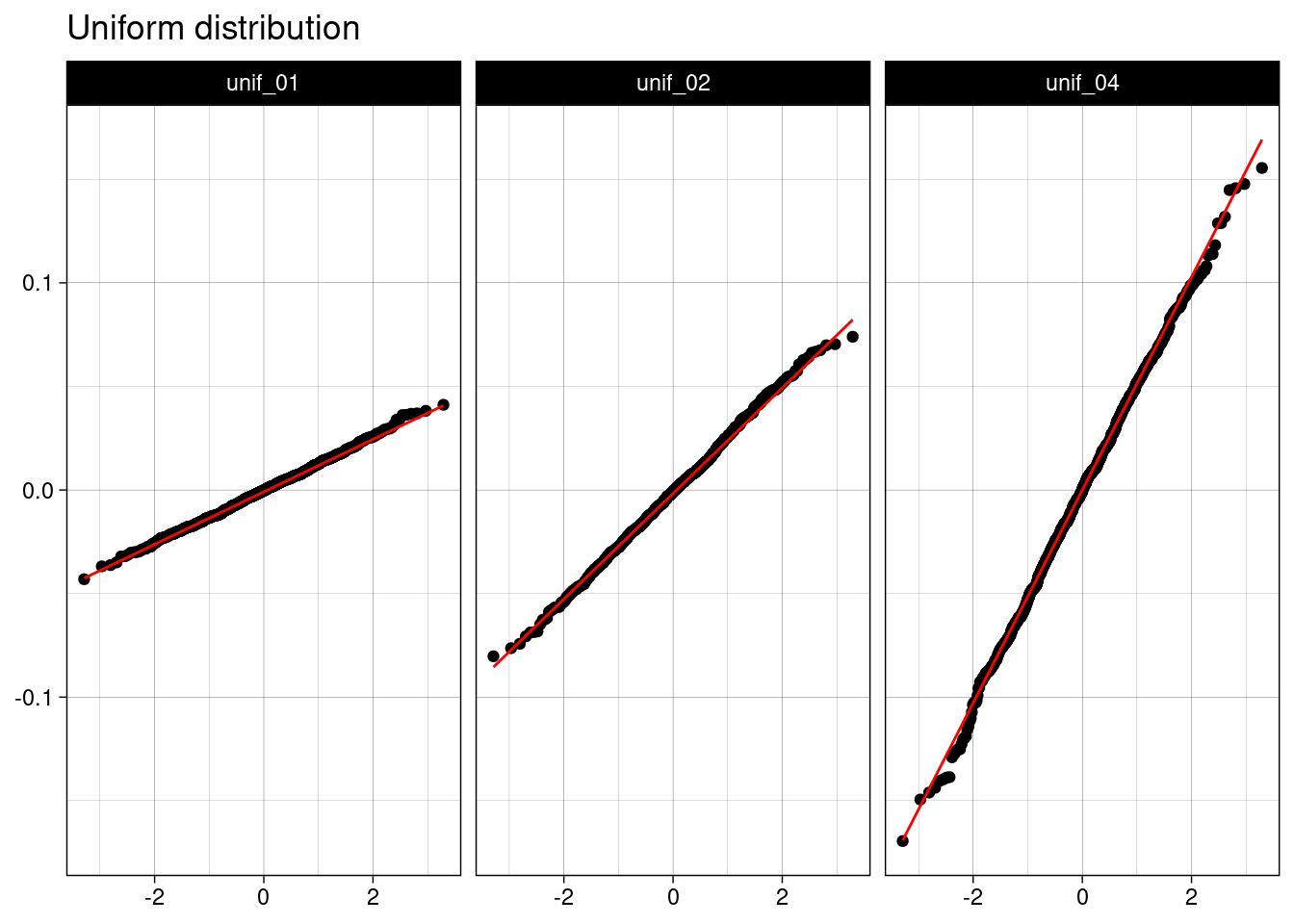
Iterating with purrr
To demonstrate empirically the central limit theorem for the normal and uniform distributions, I have used some functions of purrr to iterate along lists and vectors. The map() function works like the R base lapply() function, but others functions of the family offer additional features:
- Functions like
map_int()andmap_dbl()fix the type of the output as a vector of integer and floating point values, respectively. Thus, these functions allow controlling the type of output. - Functions like
map2()allow iterating along two inputs. Thepmap()family of functions allows iterating along multiple inputs. - Functions like
map_dfr()andmap_dfc()bind together by rows or columns the output of each iteration.
Many of the combinations of features are available in functions like map2_dfr(), so they facilitate iterating in R programming considerably.
References
- Central limit theorem https://en.wikipedia.org/wiki/Central_limit_theorem
- Q-Q plot https://en.wikipedia.org/wiki/Q%E2%80%93Q_plot
- purrr map family https://purrr.tidyverse.org/reference/index.html#map-family
Session Info
## R version 4.4.0 (2024-04-24)
## Platform: x86_64-pc-linux-gnu
## Running under: Linux Mint 21.1
##
## Matrix products: default
## BLAS:   /usr/lib/x86_64-linux-gnu/blas/libblas.so.3.10.0
## LAPACK: /usr/lib/x86_64-linux-gnu/lapack/liblapack.so.3.10.0
##
## locale:
##  [1] LC_CTYPE=es_ES.UTF-8       LC_NUMERIC=C
##  [3] LC_TIME=es_ES.UTF-8        LC_COLLATE=es_ES.UTF-8
##  [5] LC_MONETARY=es_ES.UTF-8    LC_MESSAGES=es_ES.UTF-8
##  [7] LC_PAPER=es_ES.UTF-8       LC_NAME=C
##  [9] LC_ADDRESS=C               LC_TELEPHONE=C
## [11] LC_MEASUREMENT=es_ES.UTF-8 LC_IDENTIFICATION=C
##
## time zone: Europe/Madrid
## tzcode source: system (glibc)
##
## attached base packages:
## [1] stats     graphics  grDevices utils     datasets  methods   base
##
## other attached packages:
##  [1] lubridate_1.9.3 forcats_1.0.0   stringr_1.5.1   dplyr_1.1.4
##  [5] purrr_1.0.2     readr_2.1.5     tidyr_1.3.1     tibble_3.2.1
##  [9] ggplot2_3.5.1   tidyverse_2.0.0
##
## loaded via a namespace (and not attached):
##  [1] gtable_0.3.5      jsonlite_1.8.8    highr_0.10        compiler_4.4.0
##  [5] tidyselect_1.2.1  jquerylib_0.1.4   scales_1.3.0      yaml_2.3.8
##  [9] fastmap_1.1.1     R6_2.5.1          labeling_0.4.3    generics_0.1.3
## [13] knitr_1.46        bookdown_0.39     munsell_0.5.1     tzdb_0.4.0
## [17] bslib_0.7.0       pillar_1.9.0      rlang_1.1.3       utf8_1.2.4
## [21] stringi_1.8.3     cachem_1.0.8      xfun_0.43         sass_0.4.9
## [25] timechange_0.3.0  cli_3.6.2         withr_3.0.0       magrittr_2.0.3
## [29] digest_0.6.35     grid_4.4.0        rstudioapi_0.16.0 hms_1.1.3
## [33] lifecycle_1.0.4   vctrs_0.6.5       evaluate_0.23     glue_1.7.0
## [37] farver_2.1.1      blogdown_1.19     fansi_1.0.6       colorspace_2.1-0
## [41] rmarkdown_2.26    tools_4.4.0       pkgconfig_2.0.3   htmltools_0.5.8.1