Spanish Incidence Rate of Occupational Accidents

Jose M Sallan 2025-03-18 8 min read

library(tidyverse)
library(readxl)
library(mapSpain)

The incidence rate is a measure of occupational accidents, equal to the number of accidents occurring at work and requiring a leave period per 100,000 workers exposed to the risk. In Spain, it is usually calculated for four sectors of economic activity: construction (construcción), manufacturing (industria), agriculture (agricultura) and services (servicios). In this post, we will examine the evolution of this metric across regions (comunidades autónomas) in 2013-2023 period. Doing this analysis requires:

Reading the data from an Excel file with readxl.
Handling and analyzing data with the tidyverse.
Doing choroplethic maps with mapSpain.

Reading and Processing Data

Let’s start reading the sheet ATR-I.1.3 of the ATR_2023_I.xlsx file. I need to input the lines to skip and the lines to read, to avoid headers and footnotes. Then, I remove the empty lines between blocks of data.

iind <- read_excel("ATR_2023_I.xlsx",
                   sheet = "ATR-I.1.3",
                   skip = 6,
                   n_max = 106) # 105 rows

## New names:
## • `` -> `...1`

iind <- iind |>
  filter(!is.na(`2013`)) # 95 rows

The types vector includes the Spanish name of all sectors of activity. I use this vector to create a sector column to report the sector the data belongs to, and replace the TOTAL values of region with España.

types <- c("TOTAL", "AGRARIO", "INDUSTRIA", "CONSTRUCCIÓN", "SERVICIOS")

iind <- iind |>
  mutate(sector = rep(types, each = 19)) |>
  relocate(sector, .after = ...1)

iind <- iind |>
  rename(region = ...1) |>
  mutate(region = ifelse(region %in% types, "España", region))

Finally, I am using pivot_longer() to present the data as a long table, and update the data type of year to numeric.

iind <- iind |>
  pivot_longer(-c(region, sector), names_to = "year", values_to = "index") |>
  mutate(year = as.numeric(year))
iind

## # A tibble: 1,045 × 4
##    region sector  year index
##    <chr>  <chr>  <dbl> <dbl>
##  1 España TOTAL   2013 3009.
##  2 España TOTAL   2014 3111.
##  3 España TOTAL   2015 3252.
##  4 España TOTAL   2016 3364.
##  5 España TOTAL   2017 3409.
##  6 España TOTAL   2018 3409.
##  7 España TOTAL   2019 3020.
##  8 España TOTAL   2020 2455.
##  9 España TOTAL   2021 2810.
## 10 España TOTAL   2022 2951.
## # ℹ 1,035 more rows

Analyzing Data: Temporal Evolution

Let’s create a plot representing the evolution of the incidence rate for each sector in Spain. I want to attach direct labels to the table, so I am creating the iind_dl table to position the sector name.

iind_dl <- iind |>
  group_by(sector) |>
  filter(region == "España", year == max(year))

Here is the line plot representing the evolution of the incidence rate from 2013 to 2023. Some of the modifications to the plot are:

Temporal labels are modified with scale_x_continuous(). Here I am also removing the axis title and modifying the limits of the axis to make room for the direct labels.
Direct labels are attached with geom_text() using the iind_dl data.
In the labs() function I give a title to the plot and remove the y axis label.

iind |>
  filter(region == "España") |>
  ggplot(aes(year, index, color = sector)) +
  geom_line(linewidth = 1) +
  scale_x_continuous(name = element_blank(), 
                     breaks = seq(2013, 2023, 2), 
                     limits = c(2013, 2025)) +
  labs(title = "Índice Rate of Occupational Accidents", 
       caption = "Source: MITES", y = NULL) +
  geom_text(data = iind_dl, 
            aes(year, index, color = sector, label = sector), 
            hjust = 0, show.legend = FALSE, size = 3) +
  theme_minimal() +
  scale_color_viridis_d() +
  theme(legend.position = "none")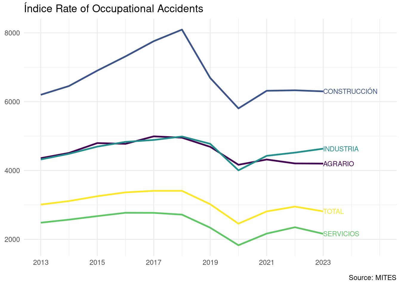

We observe that the construction sector has the highest incidence rates along the years. Agriculture and manufacturing have similar values, and services sector has the lowest incidence rates. Global levels of incidence rate are close to services because of the high weight of services in the Spanish economy. Incidence rates peaked around 2018, have a slight decrease during the COVID years and have raised slightly since then. The reduction of the incidence rates during COVID is moderate because accidents and people working on each sector lowered at a similar pace.

Analyzing Data: Regional Differences

To account for geographical differences, I have built choropleth maps with the mapSpain package. Here is a regional map of Spain using this package.

ccaa_sf <- esp_get_ccaa_siane()
can <- esp_get_can_box()
ggplot(ccaa_sf) +
  geom_sf() +
  geom_sf(data = can, color = "grey70") +
  theme_void()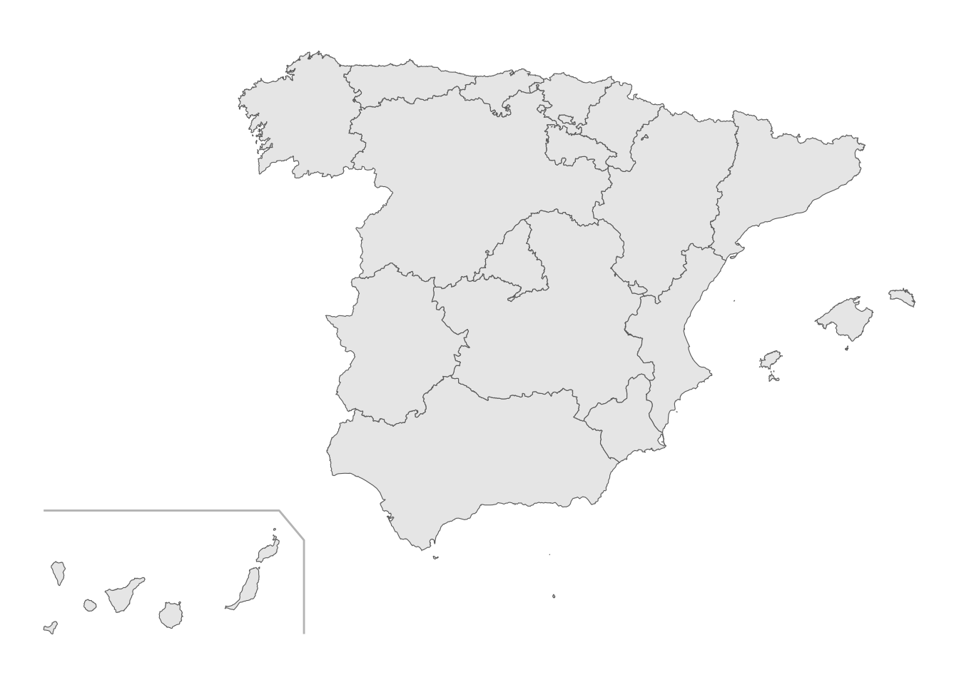

I need to bind incidence rates with regions of the map, so I need to match the iso2 codes of each region with the region names presented in the data. I am doing this with the iso_ccaa table.

iso_ccaa <- ccaa_sf$iso2.ccaa.code
tabla_ccaa <- tibble(region = unique(iind$region),
                     iso = c("ES", iso_ccaa[c(1:6, 8, 7, 9:18)]))
tabla_ccaa

## # A tibble: 19 × 2
##    region                       iso  
##    <chr>                        <chr>
##  1 España                       ES   
##  2 Andalucía                    ES-AN
##  3 Aragón                       ES-AR
##  4 Asturias (Principado de)     ES-AS
##  5 Balears (Illes)              ES-IB
##  6 Canarias                     ES-CN
##  7 Cantabria                    ES-CB
##  8 Castilla-La Mancha           ES-CM
##  9 Castilla y León              ES-CL
## 10 Cataluña                     ES-CT
## 11 Comunitat Valenciana         ES-VC
## 12 Extremadura                  ES-EX
## 13 Galicia                      ES-GA
## 14 Madrid (Comunidad de)        ES-MD
## 15 Murcia (Región de)           ES-MC
## 16 Navarra (Comunidad Foral de) ES-NC
## 17 País Vasco                   ES-PV
## 18 Rioja (La)                   ES-RI
## 19 Ceuta y Melilla              ES-CE

I use inner_join() to attach iso2 codes of regions to the data:

iind_iso <- inner_join(iind, tabla_ccaa, by = "region")

… and use left_join() to attach to the map values of incidence rates in construction in 2023.

map_constr <- left_join(ccaa_sf,
                        iind_iso |>
                          filter(sector == "CONSTRUCCIÓN", year == 2023),
                        by = c("iso2.ccaa.code" = "iso"))


ggplot(map_constr) +
  geom_sf(aes(fill = index)) +
  geom_sf(data = can, color = "grey70") +
  scale_fill_gradient(low = "#FFFF99", high = "#990000") +
  theme_void() +
  theme(legend.position = "none") +
  labs(title = "Incidence Rate in Construction (2023)")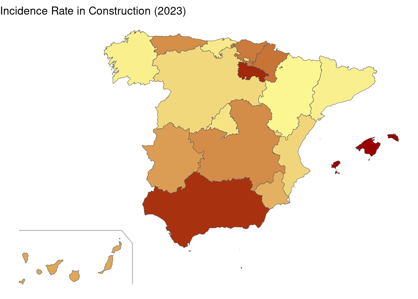

We observe that Barcelona and Madrid have moderate incidence rates. The highest values seem to correspond to Balearic Islands, La Rioja and Andalusia.

Let’s proceed in the same way with manufacturing in 2023:

map_indust <- left_join(ccaa_sf,
                        iind_iso |>
                          filter(sector == "INDUSTRIA", year == 2023),
                        by = c("iso2.ccaa.code" = "iso"))

ggplot(map_indust) +
  geom_sf(aes(fill = index)) +
  geom_sf(data = can, color = "grey70") +
  scale_fill_gradient(low = "#FFFF99", high = "#990000") +
  theme_void() +
  theme(legend.position = "none") +
  labs(title = "Incidence Rate in Manufacturing (2023)")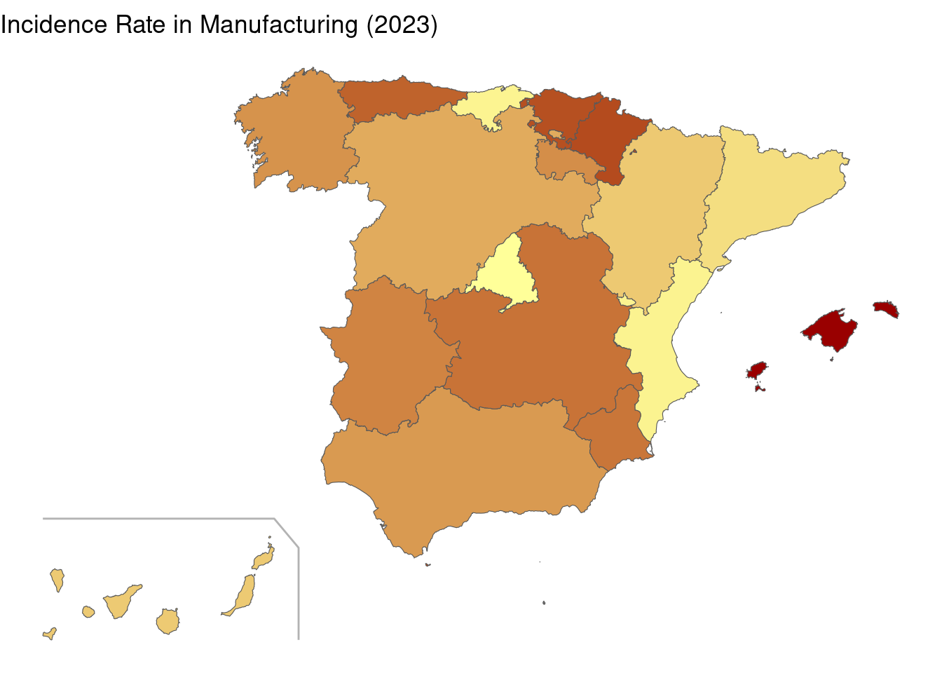

Again, Barcelona and Madrid have relatively low incidence rates. The highest values are for Balearic Islands, Basque Country and Navarre.

map_agricu <- left_join(ccaa_sf,
                        iind_iso |>
                          filter(sector == "AGRARIO", year == 2023),
                        by = c("iso2.ccaa.code" = "iso"))

ggplot(map_agricu) +
  geom_sf(aes(fill = index)) +
  geom_sf(data = can, color = "grey70") +
  scale_fill_gradient(low = "#FFFF99", high = "#990000") +
  theme_void() +
  theme(legend.position = "none") +
  labs(title = "Incidence Rate in Agriculture (2023)")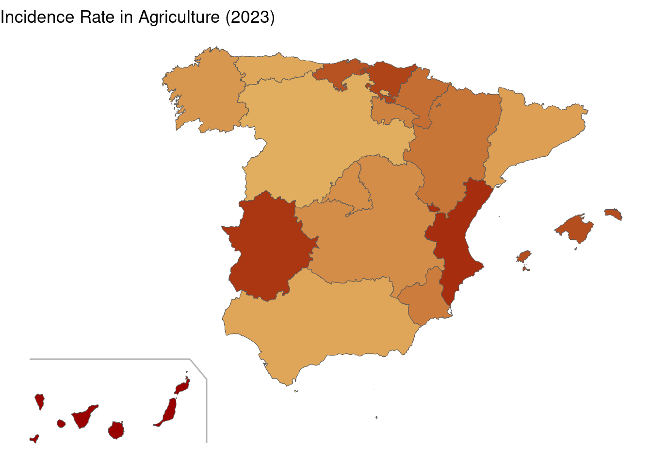

This is the mop of agriculture. Here incidence rates are more evenly distributed. The highest values are for Valencia, Extremadura, Cantabria, Basque Country, Canary Islands and Balearic Islands.

map_servic <- left_join(ccaa_sf,
                        iind_iso |>
                          filter(sector == "SERVICIOS", year == 2023),
                        by = c("iso2.ccaa.code" = "iso"))

ggplot(map_servic) +
  geom_sf(aes(fill = index)) +
  geom_sf(data = can, color = "grey70") +
  scale_fill_gradient(low = "#FFFF99", high = "#990000") +
  theme_void() +
  theme(legend.position = "none") +
  labs(title = "Incidence Rate in Services (2023)")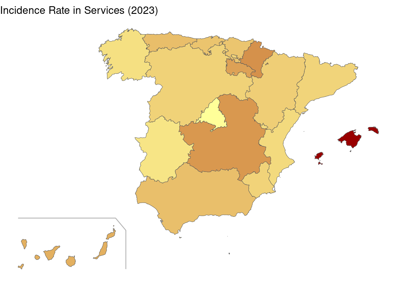

The services map is of high relevance, because it is the sector where most people are working in Spain. Here, Balearic Islands is the region with highest incidence rates.

Conclusions

From this analysis we obtain several conclusions:

Construction is the sector with highest incidence rates, followed by agriculture and manufacturing. Services has the lowest incidence rateS. Global levels of incidence rate are close to services because of the high weight of services in the Spanish economy.
Incidence rates began to lower in all sectors in 2019. The arrival of COVID reduced slightly the incidence rates, as the number of accidents reduced slightly faster than the number of people working in each sector. Since 2021, we can observe a slight increase of incidence rates.
Regarding spatial distribution, we observe that Balearic Islands is leading the statistics of incidence rates in construction, manufacturing and services.

ib_dl <- iind_iso |>
  filter(iso %in% c("ES", "ES-IB"), sector != "TOTAL") |>
  group_by(sector) |>
  filter(year == max(year))

iind_iso |>
  filter(iso %in% c("ES", "ES-IB"), sector != "TOTAL") |>
  ggplot(aes(year, index, color = iso)) +
  geom_line() +
  scale_x_continuous(name = element_blank(), 
                     breaks = seq(2013, 2023, 2), 
                     limits = c(2013, 2024)) +
  geom_text(data = ib_dl, 
            aes(year, index, color = iso, label = iso), 
            hjust = 0, show.legend = FALSE, size = 3) +
  scale_color_manual(values = c("#CC0000", "#0000CC")) +
  facet_wrap(. ~  sector, ncol = 2) +
  theme_minimal() +
  theme(legend.position = "none") +
  labs(title = "Incidence Rate in Spain (ES) and Balearics (ES-IB)", y = NULL)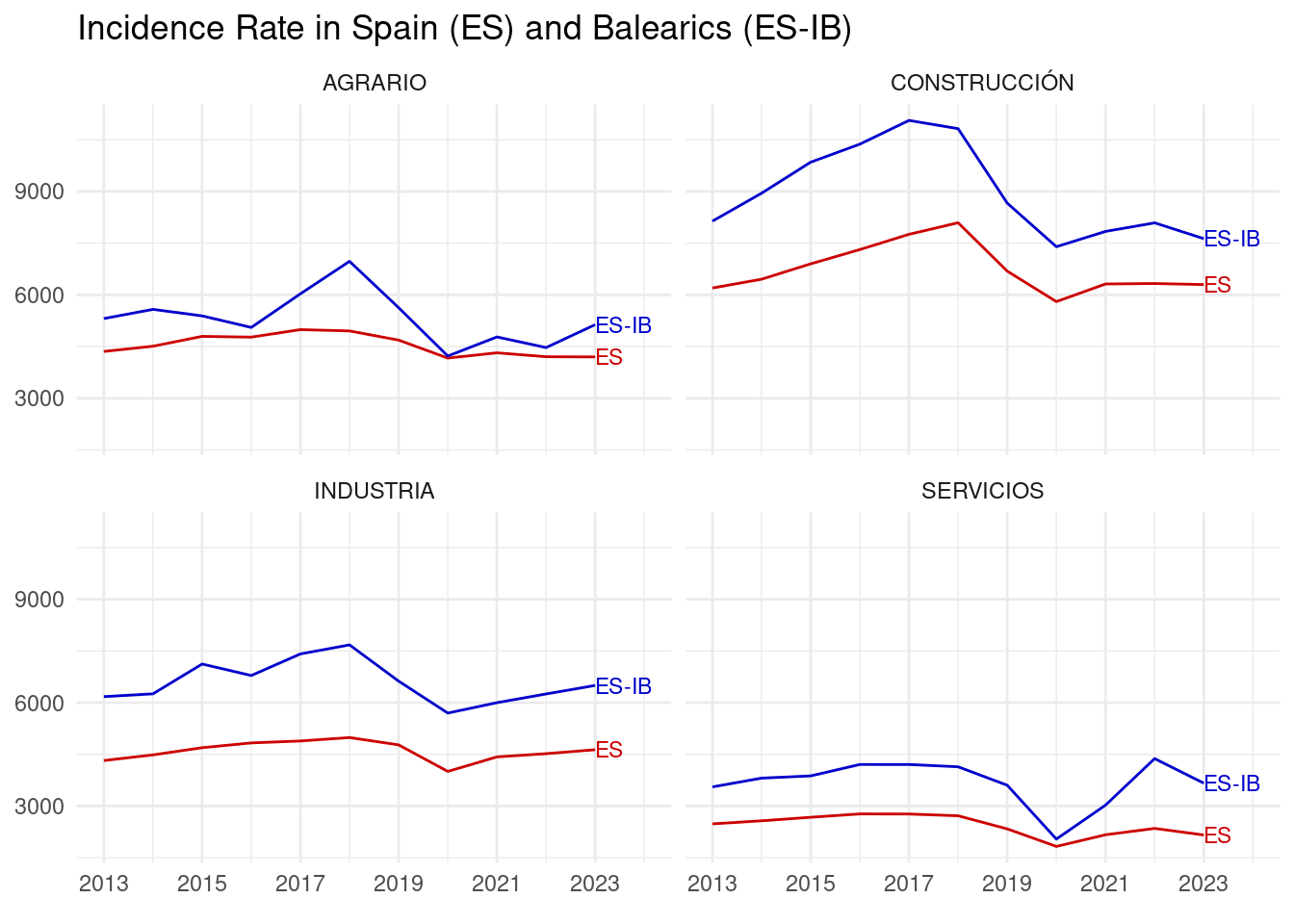

In the plot above I have compared the evolution of the incidence rate in Balearic Islands and Spain. We observe that the values in Balearic Islands are significantly higher in all sectors than in Spain. Further research is needed to account for this difference.

References

Ministerio de Trabajo y Economía Social. Estadísticas de accidentes de trabajo del año 2023. https://www.mites.gob.es/estadisticas/eat/eat23/TABLAS%20ESTADISTICAS/ATR_2023_I.xlsx
mapSpain package. https://ropenspain.github.io/mapSpain/index.html
Última Hora (2025), Baleares continúa atrapada en el ciclo de la siniestralidad laboral sin fin https://www.ultimahora.es/noticias/local/2025/01/19/2308089/trabajo-baleares-atrapados-ciclo-siniestralidad-laboral-fin.html.

All websites accessed on 2025-03-17.

Session Info

## R version 4.4.3 (2025-02-28)
## Platform: x86_64-pc-linux-gnu
## Running under: Linux Mint 21.1
## 
## Matrix products: default
## BLAS:   /usr/lib/x86_64-linux-gnu/blas/libblas.so.3.10.0 
## LAPACK: /usr/lib/x86_64-linux-gnu/lapack/liblapack.so.3.10.0
## 
## locale:
##  [1] LC_CTYPE=es_ES.UTF-8       LC_NUMERIC=C              
##  [3] LC_TIME=es_ES.UTF-8        LC_COLLATE=es_ES.UTF-8    
##  [5] LC_MONETARY=es_ES.UTF-8    LC_MESSAGES=es_ES.UTF-8   
##  [7] LC_PAPER=es_ES.UTF-8       LC_NAME=C                 
##  [9] LC_ADDRESS=C               LC_TELEPHONE=C            
## [11] LC_MEASUREMENT=es_ES.UTF-8 LC_IDENTIFICATION=C       
## 
## time zone: Europe/Madrid
## tzcode source: system (glibc)
## 
## attached base packages:
## [1] stats     graphics  grDevices utils     datasets  methods   base     
## 
## other attached packages:
##  [1] mapSpain_0.10.0 readxl_1.4.3    lubridate_1.9.4 forcats_1.0.0  
##  [5] stringr_1.5.1   dplyr_1.1.4     purrr_1.0.2     readr_2.1.5    
##  [9] tidyr_1.3.1     tibble_3.2.1    ggplot2_3.5.1   tidyverse_2.0.0
## 
## loaded via a namespace (and not attached):
##  [1] rappdirs_0.3.3     utf8_1.2.4         sass_0.4.9         generics_0.1.3    
##  [5] class_7.3-23       KernSmooth_2.23-26 blogdown_1.19      stringi_1.8.3     
##  [9] countrycode_1.6.0  hms_1.1.3          digest_0.6.35      magrittr_2.0.3    
## [13] evaluate_0.23      grid_4.4.3         timechange_0.3.0   bookdown_0.39     
## [17] fastmap_1.1.1      cellranger_1.1.0   jsonlite_1.8.9     e1071_1.7-14      
## [21] DBI_1.2.2          viridisLite_0.4.2  scales_1.3.0       jquerylib_0.1.4   
## [25] cli_3.6.2          rlang_1.1.5        units_0.8-5        munsell_0.5.1     
## [29] withr_3.0.0        cachem_1.0.8       yaml_2.3.8         tools_4.4.3       
## [33] tzdb_0.4.0         colorspace_2.1-0   vctrs_0.6.5        R6_2.5.1          
## [37] proxy_0.4-27       lifecycle_1.0.4    classInt_0.4-10    pkgconfig_2.0.3   
## [41] pillar_1.10.1      bslib_0.7.0        gtable_0.3.5       glue_1.7.0        
## [45] Rcpp_1.0.12        sf_1.0-16          highr_0.10         xfun_0.43         
## [49] tidyselect_1.2.1   rstudioapi_0.16.0  knitr_1.46         farver_2.1.1      
## [53] htmltools_0.5.8.1  labeling_0.4.3     rmarkdown_2.26     compiler_4.4.3

The Jose M Sallan static website