In this post I will introduce the use of fractional factorial designs in the evaluation of metaheuristics for combinatorial optimization problems. As an example, I will evaluate a genetic algorithm for the travelling salesman problem (TSP). In addition to the tidyverse, I will load the combheuristics package to get some TSP instances, and the FrF2 package to build fractional factorial designs.
library(tidyverse)
library(combheuristics)
library(FrF2)
To evaluate the influence of algorithm parameters on performance, we usually use experiments designed with a full factorial design. Each of the parameters to evaluate is a factor, which usually takes two different values or levels. For k factors, the number of combinations is \(2^k\). This table presents a factorial design for \(k=3\).
| A | B | C |
|---|---|---|
| -1 | -1 | -1 |
| -1 | -1 | 1 |
| -1 | 1 | -1 |
| -1 | 1 | 1 |
| 1 | -1 | -1 |
| 1 | -1 | 1 |
| 1 | 1 | -1 |
| 1 | 1 | 1 |
As the number of parameters increases, the number of different combinations of factors augments exponentially. Additionally, if the algorithm returns a random solution we need additional runs to account for variability. Then, the number of runs of an experiment can raise dramatically. A remedy for this are the fractional factorial designs. These designs are based in the principle than main effects will usually be more relevant than higher order interactions. For instance, we can generate a fractional factorial design for k=4 with the following defining relation:
\[ I = ABCD \]
This means that main effects are aliased with interactions of order three. For instance, \(D \equiv ABC\). Based on this we can create the following fractional design:
| A | B | C | D |
|---|---|---|---|
| -1 | -1 | -1 | -1 |
| -1 | -1 | 1 | 1 |
| -1 | 1 | -1 | 1 |
| -1 | 1 | 1 | -1 |
| 1 | -1 | -1 | 1 |
| 1 | -1 | 1 | -1 |
| 1 | 1 | -1 | -1 |
| 1 | 1 | 1 | 1 |
In this design, column \(D\) has been obtained multiplying columns \(A\), \(B\) and \(C\).
This fractional design is said to have resolution IV, as the length of the defining relation is equal to four. In these designs, main factors are aliased with interactions of order three, and interactions of order two with other interactions of order two.
The Genetic Algorithm
Let’s evaluate the performance of the genetic algorithm for the TSP presented in a previous post. We obtain the code for the algorithm from a Github Gist:
devtools::source_gist("https://gist.github.com/jmsallan/1d284ccc9734cc501c2400517d798cfd")## ℹ Sourcing gist "1d284ccc9734cc501c2400517d798cfd"
## ℹ SHA-1 hash of file is "84b6bae29aed049fef1da17b9b873ef75ee00533"Genetic algorithms can have a lot of parameters to tune. In this case, I am considering the following:
parameter <- c("selection", "crossover", "mutation", "pmut", "pcross", "elitist")
levels <- c("prob, tournament", "pmx, ox", "scramble, inv", "0.8, 1", "0.6, 0.3", "TRUE, FALSE")
t_grid <- tibble(factors = parameter, levels = levels)
t_grid |>
  kbl() |>
kable_styling(full_width = FALSE)| factors | levels |
|---|---|
| selection | prob, tournament |
| crossover | pmx, ox |
| mutation | scramble, inv |
| pmut | 0.8, 1 |
| pcross | 0.6, 0.3 |
| elitist | TRUE, FALSE |
The Fractional Design
If we make five runs for each combination of levels to account for solution variability we need \(2^6 \cdot 5 = 320\) runs for each instance. This can take too long, so I have used the FrF2::FrF2() function to define a fractional design of resolution III.
grid_res3 <- FrF2(factor.names = list(
  selection = c("prob", "tournament"),
  crossover = c("pmx", "ox"),
  mutation = c("scramble", "inv"),
  pcross = c(0.8, 1),
  pmut = c(0.3, 0.6),
  elitist = c("TRUE", "FALSE")
), resolution = 3, seed = 113)
The resulting table is:
grid_res3## selection crossover mutation pcross pmut elitist
## 1 prob pmx inv 1 0.3 TRUE
## 2 tournament pmx scramble 0.8 0.3 FALSE
## 3 tournament ox inv 1 0.6 FALSE
## 4 prob ox inv 0.8 0.3 FALSE
## 5 prob ox scramble 0.8 0.6 TRUE
## 6 prob pmx scramble 1 0.6 FALSE
## 7 tournament pmx inv 0.8 0.6 TRUE
## 8 tournament ox scramble 1 0.3 TRUE
## class=design, type= FrF2We have reduced the number of combinations from \(2^6 = 64\) to \(2^{\left(6-3\right)} = 8\).
The package allows obtaining the aliases of the design:
aliasprint(grid_res3)## $legend
## [1] A=selection B=crossover C=mutation D=pcross E=pmut F=elitist
##
## $main
## [1] A=BD=CE B=AD=CF C=AE=BF D=AB=EF E=AC=DF F=BC=DE
##
## $fi2
## [1] AF=BE=CDAs we can see, in this case each main factor is aliased with interactions of two factors.
Now we need to set the correct type for each column and to replicate the table five times to have five runs for each combination.
grid_res3 <- tibble(grid_res3) |>
  mutate(across(everything(), as.character)) |>
  mutate(across(pcross:pmut, as.numeric),
         elitist = as.logical(elitist))

grid <- map_dfr(1:5, ~ grid_res3 |> mutate(run = .))
The resulting grid is:
grid## # A tibble: 40 × 7
## selection crossover mutation pcross pmut elitist run
## <chr> <chr> <chr> <dbl> <dbl> <lgl> <int>
## 1 prob pmx inv 1 0.3 TRUE 1
## 2 tournament pmx scramble 0.8 0.3 FALSE 1
## 3 tournament ox inv 1 0.6 FALSE 1
## 4 prob ox inv 0.8 0.3 FALSE 1
## 5 prob ox scramble 0.8 0.6 TRUE 1
## 6 prob pmx scramble 1 0.6 FALSE 1
## 7 tournament pmx inv 0.8 0.6 TRUE 1
## 8 tournament ox scramble 1 0.3 TRUE 1
## 9 prob pmx inv 1 0.3 TRUE 2
## 10 tournament pmx scramble 0.8 0.3 FALSE 2
## # ℹ 30 more rowsTest Instances
In this experiment, I will use four benchmark instances from TSPLIB, stored in the combheuristics package.
gr24 <- TSPLIB_sample$gr24
gr48 <- TSPLIB_sample$gr48
eil76 <- TSPLIB_sample$eil76
eil101 <- TSPLIB_sample$eil101
The experimental Evaluation
Now we are ready to run the experiment. I am using the purrr::pmap_dbl() function to add the fit column to the table, assigning the values from the grid table to the algorithm.
set.seed(1313)
exp_gr24 <- grid |>
  mutate(fit = pmap_dbl(grid, ~ ga_tsp(gr24$D, npop = 200, max_iter = 300, selection = ..1, crossover = ..2, mutation = ..3, pcross = ..4, pmut = ..5, elitist = ..6)$fit))

set.seed(1313)
exp_gr48 <- grid |>
  mutate(fit = pmap_dbl(grid, ~ ga_tsp(gr48$D, npop = 200, max_iter = 300, selection = ..1, crossover = ..2, mutation = ..3, pcross = ..4, pmut = ..5, elitist = ..6)$fit))

set.seed(1313)
exp_eil76 <- grid |>
  mutate(fit = pmap_dbl(grid, ~ ga_tsp(eil76$D, npop = 400, max_iter = 600, selection = ..1, crossover = ..2, mutation = ..3, pcross = ..4, pmut = ..5, elitist = ..6)$fit))

set.seed(1313)
exp_eil101 <- grid |>
  mutate(fit = pmap_dbl(grid, ~ ga_tsp(eil101$D, npop = 400, max_iter = 600, selection = ..1, crossover = ..2, mutation = ..3, pcross = ..4, pmut = ..5, elitist = ..6)$fit))
Let’s take a look at the best values of average fit for each instance:
map(list(exp_gr24, exp_gr48, exp_eil76, exp_eil101), ~ . |>
      group_by(pick(selection:elitist)) |>
      summarise(fit = mean(fit), .groups = "drop") |>
      arrange(fit))
## [[1]]
## # A tibble: 8 × 7
## selection crossover mutation pcross pmut elitist fit
## <chr> <chr> <chr> <dbl> <dbl> <lgl> <dbl>
## 1 tournament ox inv 1 0.6 FALSE 1290.
## 2 tournament pmx inv 0.8 0.6 TRUE 1297.
## 3 prob ox inv 0.8 0.3 FALSE 1391
## 4 tournament pmx scramble 0.8 0.3 FALSE 1423.
## 5 tournament ox scramble 1 0.3 TRUE 1434.
## 6 prob pmx inv 1 0.3 TRUE 1525
## 7 prob ox scramble 0.8 0.6 TRUE 1543.
## 8 prob pmx scramble 1 0.6 FALSE 1553
##
## [[2]]
## # A tibble: 8 × 7
## selection crossover mutation pcross pmut elitist fit
## <chr> <chr> <chr> <dbl> <dbl> <lgl> <dbl>
## 1 tournament pmx inv 0.8 0.6 TRUE 5296.
## 2 tournament ox inv 1 0.6 FALSE 5453.
## 3 tournament pmx scramble 0.8 0.3 FALSE 5903.
## 4 tournament ox scramble 1 0.3 TRUE 5918
## 5 prob ox inv 0.8 0.3 FALSE 6072.
## 6 prob pmx inv 1 0.3 TRUE 6089.
## 7 prob ox scramble 0.8 0.6 TRUE 6098
## 8 prob pmx scramble 1 0.6 FALSE 6098
##
## [[3]]
## # A tibble: 8 × 7
## selection crossover mutation pcross pmut elitist fit
## <chr> <chr> <chr> <dbl> <dbl> <lgl> <dbl>
## 1 tournament pmx inv 0.8 0.6 TRUE 587.
## 2 tournament ox inv 1 0.6 FALSE 609.
## 3 tournament pmx scramble 0.8 0.3 FALSE 644.
## 4 tournament ox scramble 1 0.3 TRUE 650.
## 5 prob ox inv 0.8 0.3 FALSE 679.
## 6 prob ox scramble 0.8 0.6 TRUE 708.
## 7 prob pmx inv 1 0.3 TRUE 712.
## 8 prob pmx scramble 1 0.6 FALSE 712.
##
## [[4]]
## # A tibble: 8 × 7
## selection crossover mutation pcross pmut elitist fit
## <chr> <chr> <chr> <dbl> <dbl> <lgl> <dbl>
## 1 tournament pmx inv 0.8 0.6 TRUE 702.
## 2 tournament ox inv 1 0.6 FALSE 755.
## 3 tournament pmx scramble 0.8 0.3 FALSE 791.
## 4 tournament ox scramble 1 0.3 TRUE 801.
## 5 prob ox inv 0.8 0.3 FALSE 808.
## 6 prob pmx scramble 1 0.6 FALSE 824.
## 7 prob ox scramble 0.8 0.6 TRUE 825.
## 8 prob pmx inv 1 0.3 TRUE 825.We can see that we obtain the best values with tournament = "selection", mutation = "inv" and high values of pmut, although analyses not presented here show that the algorithm diverges for large instances when higher values of pmut are used. The parameters pcross and elitism seem to have a lesser influence on performance.
A Smaller Full Factorial Experiment
As the results of the fractional factorial are aliased with interactions of two factors, I have decided to run a full factorial experiment with the selection and mutation operators and levels of pmut as factors. I have fixed the values of the crossover operator to pmx, probability of crossover to 0.8 and set elitism to FALSE.
The grid of a full factorial can be obtained with tidyr::expand_grid():
small_grid <- expand_grid(
  selection = c("prob", "tournament"),
  mutation = c("scramble", "inv"),
  pmut = c(0.3, 0.6)
)

small_grid <- map_dfr(1:5, ~ small_grid |> mutate(run = .))
small_grid
## # A tibble: 40 × 4
## selection mutation pmut run
## <chr> <chr> <dbl> <int>
## 1 prob scramble 0.3 1
## 2 prob scramble 0.6 1
## 3 prob inv 0.3 1
## 4 prob inv 0.6 1
## 5 tournament scramble 0.3 1
## 6 tournament scramble 0.6 1
## 7 tournament inv 0.3 1
## 8 tournament inv 0.6 1
## 9 prob scramble 0.3 2
## 10 prob scramble 0.6 2
## # ℹ 30 more rowsThis grid has also 40 runs for each instance, but is focused on three factors only.
set.seed(1313)
expsg_gr24 <- small_grid |>
  mutate(fit = pmap_dbl(small_grid, ~ ga_tsp(gr24$D, npop = 200, max_iter = 300, selection = ..1, crossover = "pmx", mutation = ..2, pcross = 0.8, pmut = ..3, elitist = FALSE)$fit))

set.seed(1313)
expsg_gr48 <- small_grid |>
  mutate(fit = pmap_dbl(small_grid, ~ ga_tsp(gr48$D, npop = 200, max_iter = 300, selection = ..1, crossover = "pmx", mutation = ..2, pcross = 0.8, pmut = ..3, elitist = FALSE)$fit))

set.seed(1313)
expsg_eil76 <- small_grid |>
  mutate(fit = pmap_dbl(small_grid, ~ ga_tsp(eil76$D, npop = 400, max_iter = 600, selection = ..1, crossover = "pmx", mutation = ..2, pcross = 0.8, pmut = ..3, elitist = FALSE)$fit))

set.seed(1313)
expsg_eil101 <- small_grid |>
  mutate(fit = pmap_dbl(small_grid, ~ ga_tsp(eil101$D, npop = 400, max_iter = 600, selection = ..1, crossover = "pmx", mutation = ..2, pcross = 0.8, pmut = ..3, elitist = FALSE)$fit))
To compare results between models, I have set a norm_fit value of normalized gap respect to the optimum.
opt_values <- map_dbl(list(gr24, gr48, eil76, eil101), ~ tsp_dist(.$D, .$opt.tour))

expsg_gr24 <- expsg_gr24 |>
  mutate(norm_fit = (fit - opt_values[1])/opt_values[1])
expsg_gr48 <- expsg_gr48 |>
  mutate(norm_fit = (fit - opt_values[2])/opt_values[2])
expsg_eil76 <- expsg_eil76 |>
  mutate(norm_fit = (fit - opt_values[3])/opt_values[3])
expsg_eil101 <- expsg_eil101 |>
  mutate(norm_fit = (fit - opt_values[4])/opt_values[4])
Now we can take a look at the results:
map(list(expsg_gr24, expsg_gr48, expsg_eil76, expsg_eil101), ~ . |>
      group_by(pick(selection:pmut)) |>
      summarise(fit = mean(norm_fit), .groups = "drop") |>
      arrange(fit))
## [[1]]
## # A tibble: 8 × 4
## selection mutation pmut fit
## <chr> <chr> <dbl> <dbl>
## 1 tournament inv 0.6 0.0102
## 2 tournament inv 0.3 0.0272
## 3 prob inv 0.3 0.100
## 4 prob scramble 0.3 0.107
## 5 tournament scramble 0.6 0.110
## 6 tournament scramble 0.3 0.118
## 7 prob scramble 0.6 0.186
## 8 prob inv 0.6 0.188
##
## [[2]]
## # A tibble: 8 × 4
## selection mutation pmut fit
## <chr> <chr> <dbl> <dbl>
## 1 tournament inv 0.3 0.0354
## 2 tournament inv 0.6 0.0583
## 3 tournament scramble 0.3 0.166
## 4 tournament scramble 0.6 0.188
## 5 prob inv 0.3 0.189
## 6 prob scramble 0.3 0.199
## 7 prob inv 0.6 0.205
## 8 prob scramble 0.6 0.207
##
## [[3]]
## # A tibble: 8 × 4
## selection mutation pmut fit
## <chr> <chr> <dbl> <dbl>
## 1 tournament inv 0.3 0.0650
## 2 tournament inv 0.6 0.0746
## 3 tournament scramble 0.6 0.216
## 4 tournament scramble 0.3 0.227
## 5 prob scramble 0.3 0.273
## 6 prob inv 0.3 0.290
## 7 prob scramble 0.6 0.305
## 8 prob inv 0.6 0.305
##
## [[4]]
## # A tibble: 8 × 4
## selection mutation pmut fit
## <chr> <chr> <dbl> <dbl>
## 1 tournament inv 0.3 0.0483
## 2 tournament inv 0.6 0.0740
## 3 tournament scramble 0.6 0.206
## 4 tournament scramble 0.3 0.239
## 5 prob scramble 0.3 0.265
## 6 prob inv 0.6 0.280
## 7 prob inv 0.3 0.281
## 8 prob scramble 0.6 0.284Now we see that the best combination of parameters is selection = "tournament" together with mutation = "inv". The best results are obtained with the two operators working at the same time.
Scaling of Results
In the previous post I presented with this code, I obtained good values for the gr24 and gr48 instances using these operators with pmut=0.8. When tested on larger instances, the algorithm diverged when using high values of pmut. That is why I have used 0.6 as highest value of pmut: higher values did not scaled well for larger instances.
Let’s run the algorithm with gr24:
set.seed(11)
ga_gr24_2 <- ga_tsp(instance = gr24$D, selection = "tournament",
                  crossover = "ox", mutation = "inv", npop = 120,
                  max_iter = 263, pcross = 0.8, pmut = 0.8,
                  elitist = TRUE, seed = TRUE)
The evolution of the fitness values shows how the algorithm helps finding the optimum:
ga_gr24_2$track |>
  pivot_longer(-step) |>
  ggplot(aes(step, value, color = name)) +
  geom_line() +
  theme_minimal() +
  theme(legend.position = "bottom") +
  labs(x = NULL, y = NULL, title = "gr24 with pmut = 0.8") +
  scale_color_manual(name = "fit", values = c("#0066CC", "#3399FF", "#99CCFF" ))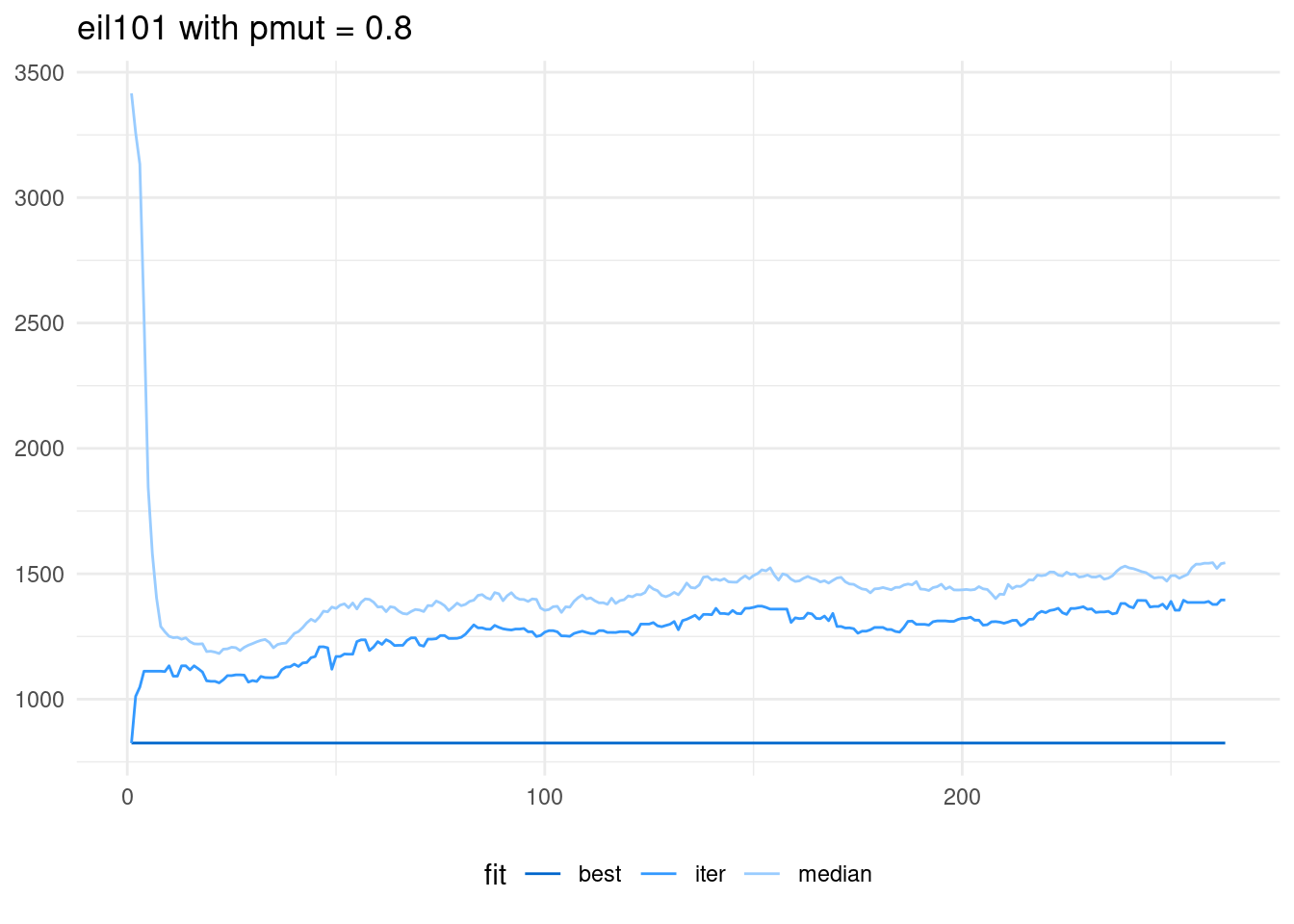
When applied the same pattern to eil101, the algorithms diverges greatly. In fact, it returns the value of the solution obtained with nearest neighbor seeded in the first generation.
set.seed(11)
ga_eil101_2 <- ga_tsp(instance = eil101$D, selection = "tournament",
                  crossover = "ox", mutation = "inv", npop = 120,
                  max_iter = 263, pcross = 0.8, pmut = 0.8,
                  elitist = TRUE, seed = TRUE)

ga_eil101_2$track |>
  pivot_longer(-step) |>
  ggplot(aes(step, value, color = name)) +
  geom_line() +
  theme_minimal() +
  theme(legend.position = "bottom") +
  labs(x = NULL, y = NULL, title = "eil101 with pmut = 0.8") +
  scale_color_manual(name = "fit", values = c("#0066CC", "#3399FF", "#99CCFF" ))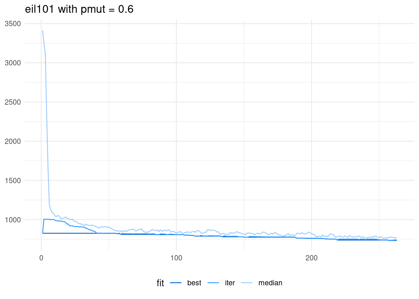
With a smaller value of pmut, the algorithm works better:
set.seed(11)
ga_eil101_3 <- ga_tsp(instance = eil101$D, selection = "tournament",
                  crossover = "ox", mutation = "inv", npop = 120,
                  max_iter = 263, pcross = 0.8, pmut = 0.6,
                  elitist = TRUE, seed = TRUE)

ga_eil101_3$track |>
  pivot_longer(-step) |>
  ggplot(aes(step, value, color = name)) +
  geom_line() +
  theme_minimal() +
  theme(legend.position = "bottom") +
  labs(x = NULL, y = NULL, title = "eil101 with pmut = 0.6") +
  scale_color_manual(name = "fit", values = c("#0066CC", "#3399FF", "#99CCFF" ))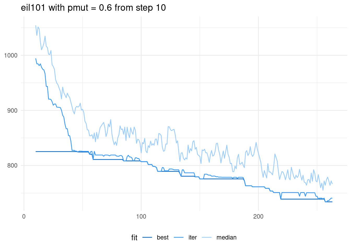
If we represent the later steps we can appreciate better how the algorithm is working.
ga_eil101_3$track |>
  pivot_longer(-step) |>
  filter(step >= 10) |>
  ggplot(aes(step, value, color = name)) +
  geom_line() +
  theme_minimal() +
  theme(legend.position = "bottom") +
  labs(x = NULL, y = NULL, title = "eil101 with pmut = 0.6 from step 10") +
  scale_color_manual(name = "fit", values = c("#0066CC", "#3399FF", "#99CCFF" ))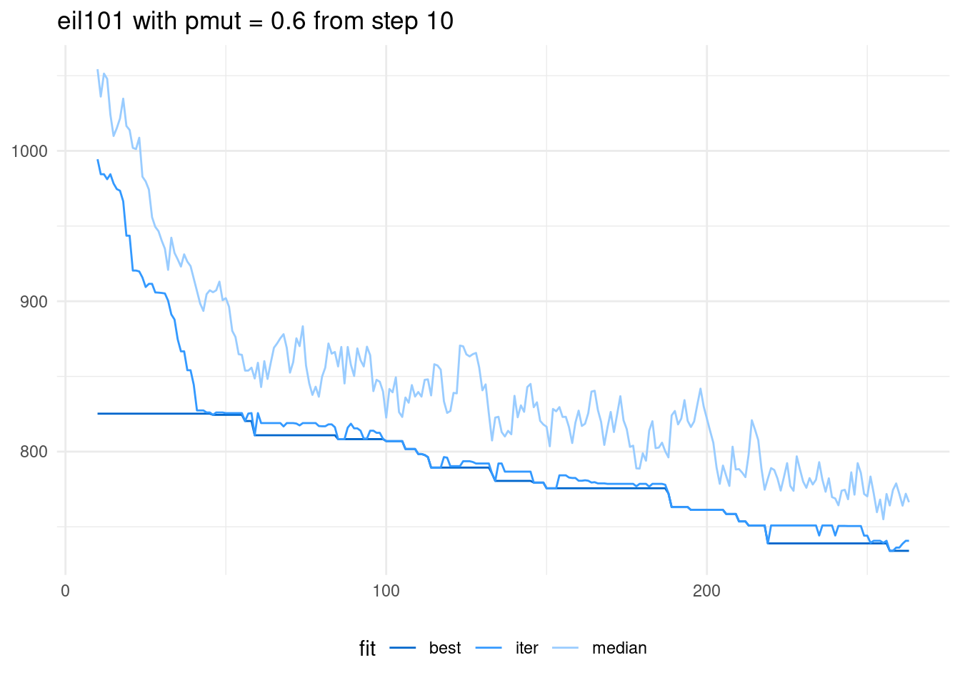
Another effect of scaling is that for larger instances we need more evaluations of the objective function to obtain stable results. As each evaluation is more costly in larger instances, the running of the algorithm in larger instances consumes significantly more time.
References
- Grömping, U. (2014). R package FrF2 for creating and analyzing fractional factorial 2-level designs. Journal of Statistical Software, 56, 1-56. https://doi.org/10.18637/jss.v056.i01.
- combheuristics package: https://github.com/jmsallan/combheuristics.
- Genetic algorithms with permutative encoding: https://jmsallan.netlify.app/blog/genetic-algorithms-with-permutative-encoding/
Session Info
## R version 4.6.0 (2026-04-24)
## Platform: x86_64-pc-linux-gnu
## Running under: Linux Mint 21.1
##
## Matrix products: default
## BLAS:   /usr/lib/x86_64-linux-gnu/blas/libblas.so.3.10.0
## LAPACK: /usr/lib/x86_64-linux-gnu/lapack/liblapack.so.3.10.0  LAPACK version 3.10.0
##
## locale:
##  [1] LC_CTYPE=es_ES.UTF-8       LC_NUMERIC=C
##  [3] LC_TIME=es_ES.UTF-8        LC_COLLATE=es_ES.UTF-8
##  [5] LC_MONETARY=es_ES.UTF-8    LC_MESSAGES=es_ES.UTF-8
##  [7] LC_PAPER=es_ES.UTF-8       LC_NAME=C
##  [9] LC_ADDRESS=C               LC_TELEPHONE=C
## [11] LC_MEASUREMENT=es_ES.UTF-8 LC_IDENTIFICATION=C
##
## time zone: Europe/Madrid
## tzcode source: system (glibc)
##
## attached base packages:
## [1] grid      stats     graphics  grDevices utils     datasets  methods
## [8] base
##
## other attached packages:
##  [1] kableExtra_1.4.0     FrF2_2.3-5           DoE.base_1.2-5
##  [4] conf.design_2.0.0    combheuristics_0.1.0 lubridate_1.9.5
##  [7] forcats_1.0.1        stringr_1.6.0        dplyr_1.2.1
## [10] purrr_1.2.2          readr_2.2.0          tidyr_1.3.2
## [13] tibble_3.3.1         ggplot2_4.0.3        tidyverse_2.0.0
##
## loaded via a namespace (and not attached):
##  [1] tidyselect_1.2.1     viridisLite_0.4.3    farver_2.1.2
##  [4] S7_0.2.2             fastmap_1.2.0        combinat_0.0-8
##  [7] gh_1.5.0             blogdown_1.23        numbers_0.9-2
## [10] digest_0.6.39        timechange_0.4.0     lifecycle_1.0.5
## [13] ellipsis_0.3.3       magrittr_2.0.5       compiler_4.6.0
## [16] rlang_1.2.0          sass_0.4.10          tools_4.6.0
## [19] igraph_2.3.1         utf8_1.2.6           yaml_2.3.12
## [22] knitr_1.51           labeling_0.4.3       pkgbuild_1.4.8
## [25] scatterplot3d_0.3-45 curl_7.1.0           xml2_1.5.2
## [28] RColorBrewer_1.1-3   pkgload_1.5.2        withr_3.0.2
## [31] partitions_1.10-9    colorspace_2.1-2     gitcreds_0.1.2
## [34] scales_1.4.0         MASS_7.3-65          cli_3.6.6
## [37] rmarkdown_2.31       generics_0.1.4       otel_0.2.0
## [40] rstudioapi_0.18.0    tzdb_0.5.0           sessioninfo_1.2.3
## [43] polynom_1.4-1        cachem_1.1.0         vctrs_0.7.3
## [46] devtools_2.5.2       jsonlite_2.0.0       bookdown_0.46
## [49] hms_1.1.4            systemfonts_1.3.2    vcd_1.4-13
## [52] jquerylib_0.1.4      glue_1.8.1           stringi_1.8.7
## [55] gtable_0.3.6         sfsmisc_1.1-24       lmtest_0.9-40
## [58] gmp_0.7-5.1          pillar_1.11.1        rappdirs_0.3.4
## [61] htmltools_0.5.9      R6_2.6.1             httr2_1.2.2
## [64] textshaping_1.0.5    Rdpack_2.6.6         evaluate_1.0.5
## [67] lattice_0.22-9       rbibutils_2.4.1      memoise_2.0.1
## [70] bslib_0.10.0         svglite_2.2.2        xfun_0.57
## [73] fs_2.1.0             zoo_1.8-15           usethis_3.2.1
## [76] pkgconfig_2.0.3