Error and Bias Prediction Metrics for Regression

Jose M Sallan 2026-02-10 8 min read

A key step in any prediction job is to assess model performance of the prediction model. In the case of regression or numerical prediction, we aim to assess to what extent a model brings a prediction ${\hat{y}}_{i}$ close to the real value of the variable $y_{i}$ . Let’s see some metrics for regression using a simple modelling of the ames dataset. The dataset is available from the modeldata package of tidymodels.

library(tidymodels)
data("ames")

As we are interested in illustrating performance metrics, I will code a very simple prediction model, based on linear regression. First, I am defining a stratified split of the dataset into train and test sets.

set.seed(22)
ames_split <- initial_split(ames, prop = 0.8, strata = "Sale_Price")

The ames_rec recipel collapses infrequent levels of factor variables, filters variables of near zero variance and variables highly correlated with other variables. The resulting fitted model is ames_lm.

ames_rec <- recipe(Sale_Price ~ ., training(ames_split)) |>
  step_other(all_nominal_predictors(), threshold = 0.1) |>
  step_nzv() |>
  step_corr(all_numeric_predictors())

lm <- linear_reg()

ames_lm <- workflow() |>
  add_recipe(ames_rec) |>
  add_model(lm) |>
  fit(training(ames_split))

The tidy structure of tidymodels functions allows defining easily an ames_pred table with the real Sale_Price values and the .pred estimates of the test set.

ames_pred <- ames_lm |>
  predict(testing(ames_split)) |>
  bind_cols(testing(ames_split)) |>
  select(Sale_Price, .pred)

Then, I can plot the predicted values versus the real values.

ames_pred |>
  ggplot(aes(Sale_Price, .pred)) +
  geom_point() +
  geom_abline(slope = 1, intercept = 0, color = "red") +
  theme_minimal(base_size = 12)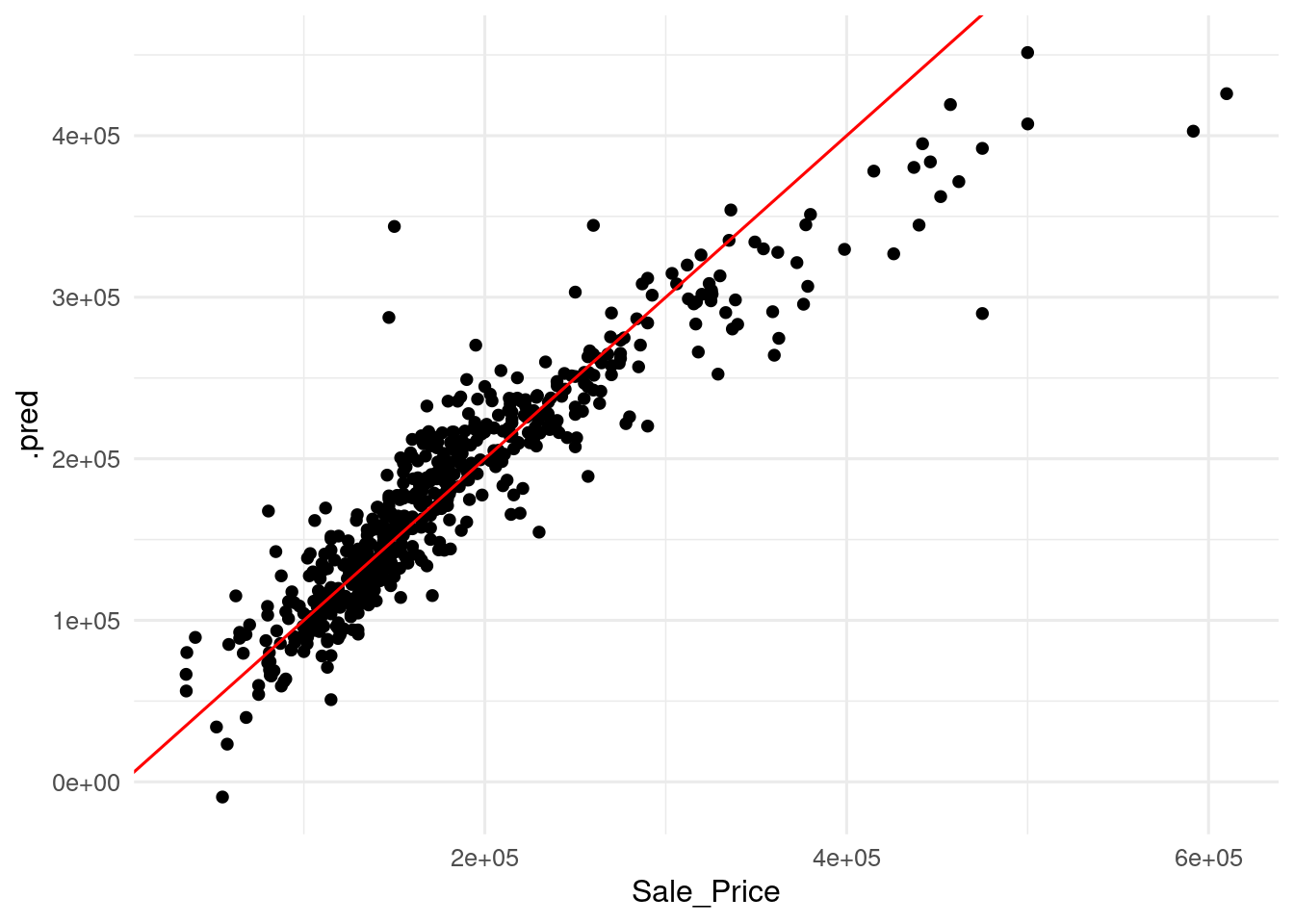

I have added a 45 degrees line, so that perfect predictions are on that line. Values over the line are overfitting, as the predicted value is larger than the real value, and values under the line are underfitting, as the predicted value is smaller than the real value.

Let’s define some metrics to asses how good a prediction like this is. These metrics will refer to two properties of the prediction:

Magnitude of error: how large is the error respect to the values of the target variable.
Bias of error: the model tends to overfit or to underfit the target variable?

Measures of Magnitude of Error

One of the most used metrics to asses magnitude of error is the root mean squared error (RMSE). Errors $y_{i} - {\hat{y}}_{i}$ are squared and averaged to make them all positive, and then the square root of the mean is extracted.

$R M S E = \sqrt{\frac{1}{n} \sum_{i = 1}^{n} {(y_{i} - {\hat{y}}_{i})}^{2}}$

To make all error terms positive, we can also take the absolute value. The resulting metric is the mean absolute error.

$M A E = \sum_{i = 1}^{n} \frac{| y_{i} - {\hat{y}}_{i} |}{n}$

Both metrics are roughly equivalent, although RMSE is more sensitive to outliers than MAPE. Then, a RMSE larger than MAPE is an indication of the presence of outliers in the prediction.

RMSE and MAPE are expressed in the units of the target variable. This can make the results hard to interpret. A remedy is using the mean absolute percentage error (MAPE). Each error is divided by the value of the target variable, so the mean is non-dimensional.

$M A P E = \frac{100}{n} \sum_{i = 1}^{n} | \frac{y_{i} - {\hat{y}}_{i}}{y_{i}} |$

Although it returns an intuitive metric of error, MAPE cannot be used with datasets where the target variable y can be zero or negative. For instance, MAPE cannot be used with temperature values if they are expressed in Celsius or Fahrenheit scales.

As the target variable must be positive, a more subtle drawback of the metric appears. While ${\hat{y}}_{i}$ cannot go below zero, it has no upper value. So MAPE can yield values larger for overestimations than for underestimations. To account for this, we can use the symmetric mean average percentage error (SMAPE). In this metric, the value of the variable is replaced by the mean of the variable and the prediction.

$S M A P E = \frac{200}{n} \sum_{i = 1}^{n} | \frac{y_{i} - {\hat{y}}_{i}}{y_{i} + {\hat{y}}_{i}} |$

The four metrics are available in yardstick, so we can define a error_metrics() function calculating these. Then, we can use if on ames_pred to obtain the metrics for our example.

error_metrics <- metric_set(rmse, mae, mape, smape)

ames_pred |>
  error_metrics(truth = Sale_Price, estimate = .pred)

## # A tibble: 4 × 3
##   .metric .estimator .estimate
##   <chr>   <chr>          <dbl>
## 1 rmse    standard     31254. 
## 2 mae     standard     20974. 
## 3 mape    standard        13.0
## 4 smape   standard        12.7

From the metrics obtained, we can estate that the prediction error of around 20,000 dollars, which is around 13% in percent. RMSE is larger than MAE, showing the presence of outliers.

Measures of Bias of Error

The metrics of bias inform if the model tens to overestimate or underestimate data. The most straight metric for bias is the mean signed deviation (MSD). It is the average value of differences $y_{i} - {\hat{y}}_{i}$ .

$M S D = \sum_{i = 1}^{n} \frac{y_{i} - {\hat{y}}_{i}}{n}$

This metric can have positive or negative values. A negative MSD means that the model tends to overestimate the target variable. A positive MSD indicates that the model tends to underestimate the target variable.

Like RMSE or MAE, MSD is expressed in the units of the target variable. To obtain a non-dimensional value of bias, we can use the mean percentage error (MPE).

$M P E = \frac{100}{n} \sum_{i = 1}^{n} \frac{y_{i} - {\hat{y}}_{i}}{y_{i}}$

MPE is subject to the same caveats than MAPE: the target variable should be strictly positive to make sense.

As with error metrics, I have created a bias_metrics() function to obtain MSD and MPE, then I have applied the function to the example.

bias_metrics <- metric_set(msd, mpe)

ames_pred |>
  bias_metrics(truth = Sale_Price, estimate = .pred)

## # A tibble: 2 × 3
##   .metric .estimator .estimate
##   <chr>   <chr>          <dbl>
## 1 msd     standard     1382.  
## 2 mpe     standard       -1.52

Interestingly, we obtain a positive value of MSD and a negative value of MPE. To examine the bias of the model, I have created a scatterplot of the deviation dev versus Sale_Price with three additional lines:

a red line on zero, separating underestimation (above) and overestimation (below).
a blue line on the value of MSD.
a trend line with geom_smooth().

ames_pred <- ames_pred |>
  mutate(dev = Sale_Price - .pred)

msd <- mean(ames_pred$dev)

ames_pred |>
  ggplot(aes(Sale_Price, dev)) +
  geom_point() +
  geom_hline(yintercept = 0, color = "red") +
  geom_hline(yintercept = msd, color = "blue") +
  geom_smooth() + 
  theme_minimal(base_size = 12)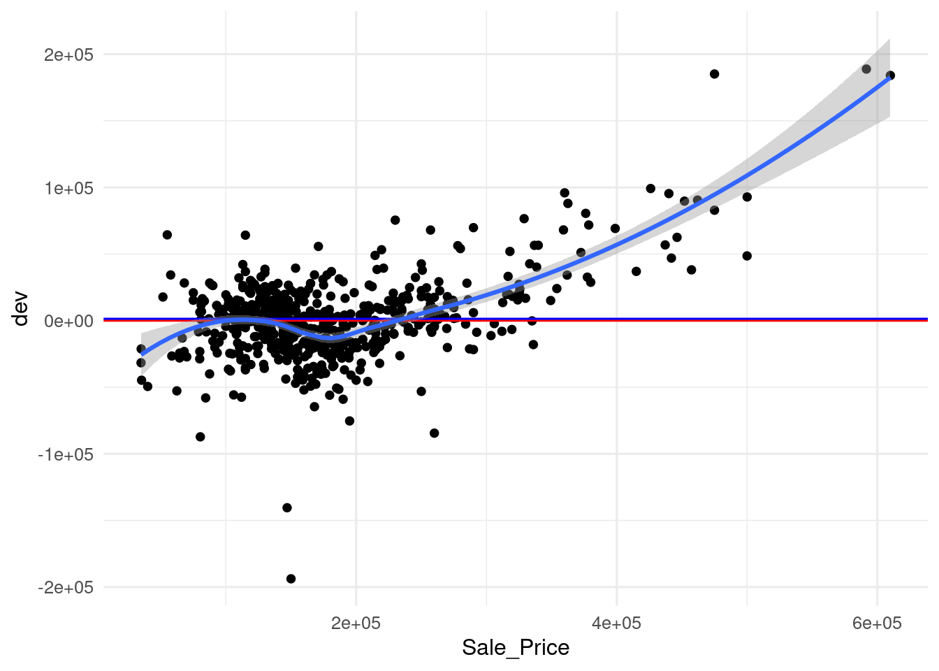

In this graph, it can be seen that the value of MSD is relatively small respect to deviations, and that the model tends to overestimate observations with small values of Sale_Price and to underestimate observations with high values.

To account for the differences between the two metrics, I have created a similar plot for deviation scaled by the target variable.

ames_pred <- ames_pred |>
  mutate(p_dev = dev/Sale_Price)

mpe <- mean(ames_pred$p_dev)

ames_pred |>
  ggplot(aes(Sale_Price, p_dev)) +
  geom_point() +
  geom_hline(yintercept = 0, color = "red") +
  geom_hline(yintercept = mpe, color = "blue") +
  geom_smooth() + 
  theme_minimal(base_size = 12)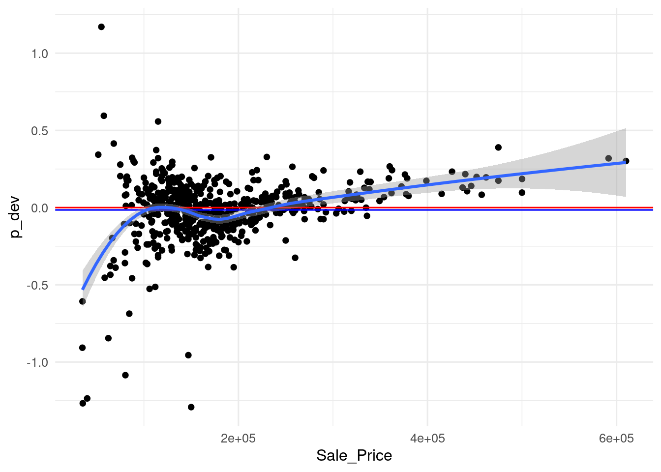

Again, here we see the same pattern as in the previous graph, but here the underestimations of expensive houses look smaller, because they have been scaled with larger values. As a result, the positive terms have a smaller weight and the metric turns negative. Nevetheless, the value of the metric is of -1.52% (the value of the graph for the metric is -0.0152), so the bias reported by the metrics is quite small. This case is another example of the explanatory power of graphical representations, when they are possible to obtain, respect to metrics.

Reference

Metrics available in the yardstick package: https://yardstick.tidymodels.org/reference/index.html
Symmetric mean absolute percentage error Wikipedia article https://en.wikipedia.org/wiki/Symmetric_mean_absolute_percentage_error

Session Info

## R version 4.5.2 (2025-10-31)
## Platform: x86_64-pc-linux-gnu
## Running under: Linux Mint 21.1
## 
## Matrix products: default
## BLAS:   /usr/lib/x86_64-linux-gnu/blas/libblas.so.3.10.0 
## LAPACK: /usr/lib/x86_64-linux-gnu/lapack/liblapack.so.3.10.0  LAPACK version 3.10.0
## 
## locale:
##  [1] LC_CTYPE=es_ES.UTF-8       LC_NUMERIC=C              
##  [3] LC_TIME=es_ES.UTF-8        LC_COLLATE=es_ES.UTF-8    
##  [5] LC_MONETARY=es_ES.UTF-8    LC_MESSAGES=es_ES.UTF-8   
##  [7] LC_PAPER=es_ES.UTF-8       LC_NAME=C                 
##  [9] LC_ADDRESS=C               LC_TELEPHONE=C            
## [11] LC_MEASUREMENT=es_ES.UTF-8 LC_IDENTIFICATION=C       
## 
## time zone: Europe/Madrid
## tzcode source: system (glibc)
## 
## attached base packages:
## [1] stats     graphics  grDevices utils     datasets  methods   base     
## 
## other attached packages:
##  [1] yardstick_1.3.2    workflowsets_1.1.0 workflows_1.2.0    tune_1.3.0        
##  [5] tidyr_1.3.1        tibble_3.3.0       rsample_1.3.0      recipes_1.3.0     
##  [9] purrr_1.2.0        parsnip_1.3.1      modeldata_1.4.0    infer_1.0.8       
## [13] ggplot2_4.0.0      dplyr_1.1.4        dials_1.4.0        scales_1.4.0      
## [17] broom_1.0.10       tidymodels_1.3.0  
## 
## loaded via a namespace (and not attached):
##  [1] tidyselect_1.2.1    timeDate_4041.110   farver_2.1.2       
##  [4] S7_0.2.0            fastmap_1.2.0       blogdown_1.21      
##  [7] digest_0.6.37       rpart_4.1.24        timechange_0.3.0   
## [10] lifecycle_1.0.4     survival_3.8-6      magrittr_2.0.4     
## [13] compiler_4.5.2      rlang_1.1.6         sass_0.4.10        
## [16] tools_4.5.2         utf8_1.2.4          yaml_2.3.10        
## [19] data.table_1.17.8   knitr_1.50          labeling_0.4.3     
## [22] DiceDesign_1.10     RColorBrewer_1.1-3  withr_3.0.2        
## [25] nnet_7.3-20         grid_4.5.2          sparsevctrs_0.3.3  
## [28] future_1.40.0       globals_0.17.0      iterators_1.0.14   
## [31] MASS_7.3-65         cli_3.6.4           rmarkdown_2.29     
## [34] generics_0.1.3      rstudioapi_0.17.1   future.apply_1.11.3
## [37] cachem_1.1.0        splines_4.5.2       parallel_4.5.2     
## [40] vctrs_0.6.5         hardhat_1.4.1       Matrix_1.7-4       
## [43] jsonlite_2.0.0      bookdown_0.43       listenv_0.9.1      
## [46] foreach_1.5.2       gower_1.0.2         jquerylib_0.1.4    
## [49] glue_1.8.0          parallelly_1.43.0   codetools_0.2-19   
## [52] lubridate_1.9.4     gtable_0.3.6        GPfit_1.0-9        
## [55] pillar_1.11.1       furrr_0.3.1         htmltools_0.5.8.1  
## [58] ipred_0.9-15        lava_1.8.1          R6_2.6.1           
## [61] lhs_1.2.0           evaluate_1.0.3      lattice_0.22-5     
## [64] backports_1.5.0     bslib_0.9.0         class_7.3-23       
## [67] Rcpp_1.1.0          nlme_3.1-168        prodlim_2024.06.25 
## [70] mgcv_1.9-4          xfun_0.52           pkgconfig_2.0.3

The Jose M Sallan static website

Error and Bias Prediction Metrics for Regression

Measures of Magnitude of Error

Measures of Bias of Error

Reference

Session Info