Computing Efficiency using igraph

Let’s use the igraph library, together with igraphdata to retrieve sample networks and the tidyverse for data handling and plotting.

library(igraph)
library(igraphdata)
library(tidyverse)
library(patchwork)
library(kableExtra)

The efficiency of a network graph can be obtained with the igraph::global_efficiency() function. We can use this function to calculate local efficiency as the average efficiency of neighbour subgraphs of network nodes with the lm_average_local_efficiency function.

lm_average_local_efficiency <- function(g){
  
  nodes <- V(g)
  
  node_ef <- sapply(nodes, \(x){
    sg <- subgraph(g, neighbors(g, x))
    e0 <- global_efficiency(sg)
    e <- ifelse(is.nan(e0), 0, e0)
    return(e)
  })
  
  lm_e <- mean(node_ef)
  
  return(lm_e)
  
}

The igraph::average_local_efficiency() function computes local efficiency with the definition of the Vragovic et al. (2005) paper. These authors define the efficiency of the neighbour subgraph of node \(i\) with paths including the full network topology cutting off only node \(i\).

Efficiency of Lattices and Random Networks

Let’s examine how evolves network efficiency for networks of the same average degree as network size increases. To calculate network parameters for lattice, Watts-Strogatz and random networks I will be using the network_measures() function, that uses the lm_average_local_efficiency() defined previously.

network_measures <- function(type = "random", n, av_degree, sample, p_rewiring = 0){
  
  m <- map_dfr(1:sample, ~{
    
    if(type == "random")
      g <- erdos.renyi.game(n = n, p.or.m = av_degree*n/2, type = "gnm", directed = FALSE)
    
    if(type == "ws")
      g <- sample_smallworld(dim = 1, size = n, nei = round(av_degree/2), p = all_of(p_rewiring))
    
    t <-  data.frame(L = mean_distance(g, unconnected = TRUE),
                     C = transitivity(g, type = "average"),
                     E_global = global_efficiency(g, directed = FALSE),
                     E_locallm = lm_average_local_efficiency(g))
    return(t)
  })
  
  meas <- m |>
    summarise(across(everything(), mean)) |>
    mutate(N = n,
           E = av_degree*n/2,
           graph = type,
           p = p_rewiring) |>
    select(graph, N, E, p, L, C, E_global, E_locallm)
  
  return(meas)
  
}

Let’s calculate network parameters for a set of networks of average degree equal to 4 and various network sizes. The values for random networks are averages across ten samples for each network size.

Ns <- seq(100, 1000, by = 100)

table_lattice <- map_dfr(Ns, ~ network_measures(type = "ws", n = ., av_degree = 4, sample = 1))

## Warning: Using `all_of()` outside of a selecting function was deprecated in tidyselect
## 1.2.0.
## ℹ See details at
##   <https://tidyselect.r-lib.org/reference/faq-selection-context.html>
## This warning is displayed once every 8 hours.
## Call `lifecycle::last_lifecycle_warnings()` to see where this warning was
## generated.

table_lattice <- table_lattice |>
  mutate(graph = "regular")

set.seed(1111)
table_random <- map_dfr(Ns, ~ network_measures(type = "random", n = ., av_degree = 4, sample = 10))

table_all <- bind_rows(table_lattice, table_random)

With this plot, I am recalling the behaviour of \(L\) and \(C\) as network size grows for regular and random networks:

• In random networks, characteristic path length grows logartihmically with \(N\), \(L \sim ln N / ln \langle k \rangle\), where \(\langle k \rangle\) is the average degree. Clustering coefficient vanishes with size \(C \sim \langle k \rangle/ N\).
• In regular networks, characteristic path length grows linearly with \(N\) while clustering coefficient remains constant with \(N\).

plotL <- table_all |>
  mutate(graph = fct_relevel(graph, "regular", "random")) |>
  ggplot(aes(N, L)) +
  geom_point() +
  scale_x_continuous(breaks = seq(100, 1000, by = 100)) +
  facet_grid(graph ~  ., scales = "free") +
  theme_bw()

plotC <- table_all |>
  mutate(graph = fct_relevel(graph, "regular", "random")) |>
  ggplot(aes(N, C)) +
  geom_point() +
  scale_x_continuous(breaks = seq(100, 1000, by = 100)) +
  facet_grid(graph ~  ., scales = "free") +
  theme_bw()

plotL + plotC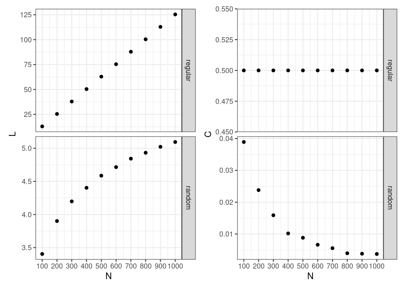

Here we have an analogous plot with global and local efficiency:

• In random networks, global and local efficiency tends to zero as network size increases.
• In regular networks, global efficiency tends to zero as network size increases. Note how the starting value of efficiency for regular networks is higher than for random networks. Local efficiency remains independent of network size.

plot_global <- table_all |>
  mutate(graph = fct_relevel(graph, "regular", "random")) |>
  ggplot(aes(N, E_global)) +
  geom_point() +
  scale_x_continuous(breaks = seq(100, 1000, by = 100)) +
  facet_grid(graph ~  ., scales = "free") +
  theme_bw()

plot_local <- table_all |>
  mutate(graph = fct_relevel(graph, "regular", "random")) |>
  ggplot(aes(N, E_locallm)) +
  geom_point() +
  scale_x_continuous(breaks = seq(100, 1000, by = 100)) +
  facet_grid(graph ~  ., scales = "free") +
  theme_bw()

plot_global + plot_local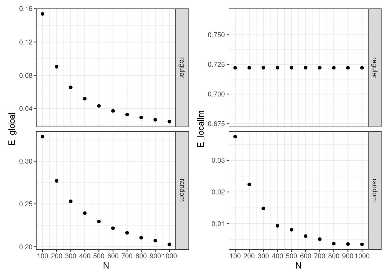

Modelling the Small-World Property

Let’s reoproduce the experiment of Watts & Strogatz (1998) to see how probabilistic rewiring of a regular lattice can produce networks with the small-world property.

p <- c(0, rep(10^{seq(-4, 0, length.out = 15)}, 20))

sm_values <- map_dfr(p, ~ network_measures(type = "ws", n = 1000, av_degree = 10, sample = 1, p_rewiring = .))

Here is a replication of the original Watts & Strogatz (1998) plot with values of \(L\) and \(C\) normalized to values for \(p=0\). We can observe a range of values of probability of rewiring with low values of \(L\) and high clustering coefficient \(C\).

scale_sm_values <- sm_values |>
  filter(p == 0)

sm_values |>
  group_by(p) |>
  summarise(across(L:C, mean)) |>
  mutate(L = L/scale_sm_values$L,
         C = C/scale_sm_values$C) |>
  filter(p != 0) |>
  pivot_longer(-p) |>
  ggplot(aes(p, value, color = name)) +
  scale_x_log10() +
  geom_point(size = 2) +
  scale_color_manual(name = "measure", labels = c("C/C(0)", "L/L(0)"), values = c("#FF8000", "#0080FF")) +
  theme_minimal() +
  labs(y = element_blank()) +
  theme(legend.position = c(0.9, 0.9))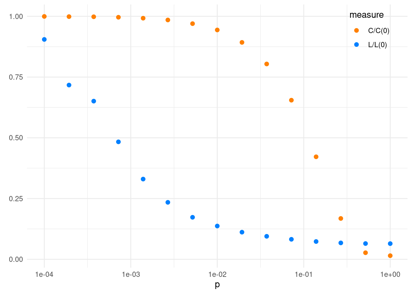

In the following plot, I am presenting the values of global and local efficiency for the same networks. For \(p \sim 0.1\) we observe how are coexisting high values of global and local efficiency.

sm_values |>
  filter(p != 0) |>
  group_by(p) |>
  summarise(across(E_global:E_locallm, mean)) |>
  pivot_longer(-p) |>
  ggplot(aes(p, value, color = name)) +
  scale_x_log10() +
  geom_point(size = 2) +
  scale_color_manual(name = "measure", labels = c(expression(E[global]), expression(E[local])), values = c("#FF8000", "#0080FF")) +
  theme_minimal() +
  labs(y = element_blank()) +
  theme(legend.position = c(0.9, 0.9))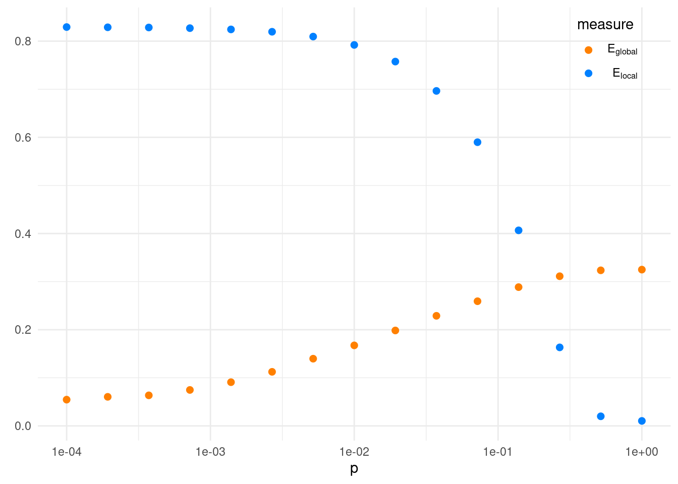

Efficiency of Real-World Networks

We can use global and local efficiency to examine if real-world networks have the small-world property. Here I will be examining the USairports network in igraphdata. As efficiency can be computed for unconnected networks, here I will retain the whole network. I will use igraph::simplify() to remove multiple edges between nodes and igraph::as.undirected() to make the network undirected.

data("USairports")
us_airports <- igraph::simplify(USairports)
us_airports <- as.undirected(us_airports)

As a benchmark, I will compute global and local efficiency for a sample of random networks with the same value of nodes and edges.

us_airports_nodes <- length(V(us_airports))
us_airports_edges <- length(E(us_airports))
us_airports_av_degree <- 2*us_airports_edges/us_airports_nodes


us_airports_random <- network_measures(type = "random", n = us_airports_nodes, av_degree = us_airports_av_degree, sample = 10)

us_airports_random <- us_airports_random |>
  select(graph, N, E, E_global, E_locallm)

us_airports_eff <- data.frame(graph = "US airports",
                              N = length(V(us_airports)),
                              E = length(E(us_airports)),
                              E_global = global_efficiency(us_airports),
                              E_locallm = lm_average_local_efficiency(us_airports))

us_airports_table <- bind_rows(us_airports_eff, us_airports_random)

us_airports_table |>
  kbl(digits = 3) |>
  kable_styling(full_width = FALSE)

We can see how the unweighted, undirected US airport network has a global efficiency of similar magnitude of a random netwok, but much higher local efficiency. Thus we can conclude that the US airport network has the small-world property.

Global and Local Efficiency of Unweighted Networks

Watts & Strogatz (1998) defined the small-world property as having a small average path length and a high average clustering coefficient. The coexistence of this global and local property was not present in regular or random networks, so they defined the Watts and Strogatz network model, consisting of rewiring randomly some edges of a regular network. For a range of values of the probability or rewiring, the Watts and Strogatz model has the small-world property.

Latora & Marchiori (2001) offered an alternative definition of the small-world property based on the global and local efficiency of transmission of information: global efficiency measures how good is the network transmitting information, and local efficiency how fault tolerant to the removal of a single node is the network. Networks with the small-world property will have high values of global and local efficiency. While average path lenght diverges for unconnected networks, global and local efficiency do not, so these metrics can be used for unconnected, unweighted networks.

References

• Latora, V. & Marchiori, M. (2001). Efficient behavior of small-world networks. Physical Review Letters, 87, 198701. https://doi.org/10.1103/PhysRevLett.87.198701
• Vragović, I., Louis, E & Díaz-Guilera, A. (2005). Efficiency of informational transfer in regular and complex networks. Physical Review E, 71, 036122. https://doi.org/10.1103/PhysRevE.71.036122
• Watts, D. J., & Strogatz, S. H. (1998). Collective dynamics of “small-world” networks. Nature, 393(6684), 440–442. https://doi.org/10.1038/30918

Session Info

## R version 4.3.1 (2023-06-16)
## Platform: x86_64-pc-linux-gnu (64-bit)
## Running under: Linux Mint 21.1
## 
## Matrix products: default
## BLAS:   /usr/lib/x86_64-linux-gnu/blas/libblas.so.3.10.0 
## LAPACK: /usr/lib/x86_64-linux-gnu/lapack/liblapack.so.3.10.0
## 
## locale:
##  [1] LC_CTYPE=es_ES.UTF-8       LC_NUMERIC=C              
##  [3] LC_TIME=es_ES.UTF-8        LC_COLLATE=es_ES.UTF-8    
##  [5] LC_MONETARY=es_ES.UTF-8    LC_MESSAGES=es_ES.UTF-8   
##  [7] LC_PAPER=es_ES.UTF-8       LC_NAME=C                 
##  [9] LC_ADDRESS=C               LC_TELEPHONE=C            
## [11] LC_MEASUREMENT=es_ES.UTF-8 LC_IDENTIFICATION=C       
## 
## time zone: Europe/Madrid
## tzcode source: system (glibc)
## 
## attached base packages:
## [1] stats     graphics  grDevices utils     datasets  methods   base     
## 
## other attached packages:
##  [1] kableExtra_1.3.4 patchwork_1.1.2  lubridate_1.9.2  forcats_1.0.0   
##  [5] stringr_1.5.0    dplyr_1.1.2      purrr_1.0.1      readr_2.1.4     
##  [9] tidyr_1.3.0      tibble_3.2.1     ggplot2_3.4.2    tidyverse_2.0.0 
## [13] igraphdata_1.0.1 igraph_1.4.2    
## 
## loaded via a namespace (and not attached):
##  [1] sass_0.4.5        utf8_1.2.3        generics_0.1.3    xml2_1.3.4       
##  [5] blogdown_1.16     stringi_1.7.12    hms_1.1.3         digest_0.6.31    
##  [9] magrittr_2.0.3    timechange_0.2.0  evaluate_0.20     grid_4.3.1       
## [13] bookdown_0.33     fastmap_1.1.1     jsonlite_1.8.4    httr_1.4.5       
## [17] rvest_1.0.3       fansi_1.0.4       viridisLite_0.4.1 scales_1.2.1     
## [21] jquerylib_0.1.4   cli_3.6.1         crayon_1.5.2      rlang_1.1.0      
## [25] munsell_0.5.0     withr_2.5.0       cachem_1.0.7      yaml_2.3.7       
## [29] tools_4.3.1       tzdb_0.3.0        colorspace_2.1-0  webshot_0.5.4    
## [33] vctrs_0.6.2       R6_2.5.1          lifecycle_1.0.3   pkgconfig_2.0.3  
## [37] pillar_1.9.0      bslib_0.5.0       gtable_0.3.3      glue_1.6.2       
## [41] systemfonts_1.0.4 highr_0.10        xfun_0.39         tidyselect_1.2.0 
## [45] rstudioapi_0.14   knitr_1.42        farver_2.1.1      htmltools_0.5.5  
## [49] labeling_0.4.2    svglite_2.1.1     rmarkdown_2.21    compiler_4.3.1