PERT (Program Evaluation and Review Technique) is a project management tool used to schedule, organize, and coordinate tasks within a project. It was developed in the 1950s for the U.S. Navy’s Polaris missile project. PERT is widely used in industries like construction, engineering, research and development, and software development, where tasks have variable duration and projects are complex.
Carrying out a PERT analysis requires:
- Breaking the project into smaller tasks or activities.
- Identifying the sequence in which tasks need to be completed and their interdependence. This requires finding the immediate predecessors of each task.
PERT analysis allows us to obtain:
- The expected time to finish the project.
- The sequence of tasks that has the longest duration, which dictates the project’s time of completion. This sequence is the critical path.
In this post, I will present how to use linear programming to obtain the expected time and critical path of a project in two contexts:
- Deterministic planning, where the time of each activity is fixed.
- Stochastic planning, where the time of a subset of all activities shows variability, and therefore follows a probability distribution. Stochastic planning is usually carried out through Monte Carlo simulation.
I will be using Rglpk for linear programming and mc2d for Monte Carlo simulation. The rest of packages are for data handling and plotting.
library(tidyverse)
library(kableExtra)
library(Rglpk)
library(mc2d)
Deterministic Planning
The following table shows an example of deterministic planning of a project with six activities with fixed time of execution.
pert <- data.frame(
  Activity = letters[1:6],
  Precedessors = c("--", "a", "--", "c", "b, d", "c"),
  Time = c(400, 600, 500, 600, 400, 900)
)

pert |>
  kbl() |>
kable_styling(full_width = FALSE)| Activity | Precedessors | Time |
|---|---|---|
| a | – | 400 |
| b | a | 600 |
| c | – | 500 |
| d | c | 600 |
| e | b, d | 400 |
| f | c | 900 |
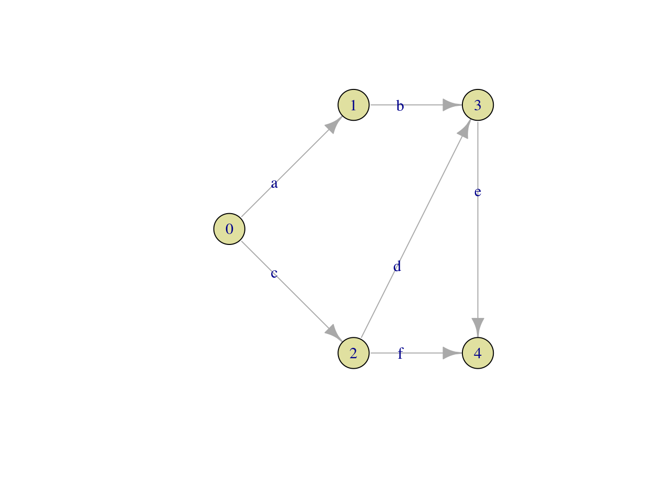
With this table of activities and predecessors we can construct the PERT chart. This chart is a graph where edges are activities and nodes are milestones. A milestone is a moment in time when one or more activities start or end.
library(igraph)
pert_df <- data.frame(orig = c(0, 1, 0, 2, 3, 2),
                      dest = c(1, 3, 2, 3, 4, 4),
                      labels = letters[1:6])

pert_graph <- graph_from_data_frame(pert_df)

pert_layout <- matrix(c(1, 2,
                        2, 3,
                        2, 1,
                        3, 3,
                        3, 1), ncol = 2, byrow = TRUE)

plot(pert_graph, layout = pert_layout, edge.label = pert_df$labels,
     vertex.size = 25, vertex.color = "#E0E0A0")
I have used the igraph library to plot the PERT chart for this project. The starting of the project is at milestone 0, and the end of the project at milestone 4.
Once defined the PERT chart, the duration of this project can be determined with a linear programming formulation with the following components:
- Decision variables: one for each milestone, representing the minimum time to reach it, considered the duration of activities.
- Constraints: one for each activity, relating its ending time with its immediate predecessors.
- Objective function: equal to the minimum time to reach the ending milestone.
For this specific project, we define four decision variables \(x_1\) to \(x_4\) for each milestone. The resulting linear programming formulation to find the project expected time is:
\[\begin{align} \text{MIN } & z = x_4 \\ \text{s. t.} & x_1 \geq 400 \\ & x_3 - x_1 \geq 600 \\ & x_2 \geq 500 \\ & x_3 - x_2 \geq 600 \\ & x_4 - x_3 \geq 400 \\ & x_4 - x_2 \geq 900 \\ & x_i \geq 0 \end{align}\]
Let’s use Rglpk to solve this problem. The solution is stored in the sol variable. Note how I am obtaining the right-hand side values of the formulation from the Time column of the pert table.
obj <- c(0, 0, 0, 1)
mat <- matrix(c(1, 0, 0, 0,
              -1, 0, 1, 0,
              0, 1, 0, 0,
              0, -1, 1, 0,
              0, 0, -1, 1,
              0, -1, 0, 1), nrow = 6, byrow = TRUE)
dir <- rep(">=", 6)
rhs <- pert$Time
max <- FALSE

sol <- Rglpk_solve_LP(obj = obj, mat = mat, dir = dir, rhs = rhs, max = max)
The value of the objective function at the optimum is the expected time to finish the project:
sol$optimum## [1] 1500To obtain the critical path we can examine the dual prices of the constraints. The activities with constraints with non-zero dual prices will form the critical path. In this formulation, a non-zero dual price for the constraint means that increasing the duration of the activity associated to the constraint will increase the expected time to finish the project.
sol$auxiliary$dual## [1] 0 0 1 1 1 0letters[which(sol$auxiliary$dual == 1)]## [1] "c" "d" "e"Then, for this problem we obtain that:
- The expected time to finish the project is 1500.
- The critical path of the project includes activities
c,dande.
Stochastic Planning
In the stochastic project planning, the duration of activities is not deterministic, but follows a probability distribution. In this case, activities duration follow a PERT distribution with the following parameters:
Min: minimum expected time to finish the activity (optimistic).Mode: most frequent expected time to finish the activity.Max: maximum expected time to finish the activity (pessimistic).
In this example, the predecessors of activities are the same as in the example of the deterministic case.
pert_random <- data.frame(
  Activity = letters[1:6],
  Precedessors = c("--", "a", "--", "c", "b, d", "c"),
  Min = c(300, 400, 250, 300, 300, 700),
  Mode = c(400, 600, 500, 600, 400, 900),
  Max = c(600, 750, 550, 700, 500, 1100),
  Distribution = rep("PERT", 6)
)

pert_random |>
  kbl() |>
kable_styling(full_width = FALSE)| Activity | Precedessors | Min | Mode | Max | Distribution |
|---|---|---|---|---|---|
| a | – | 300 | 400 | 600 | PERT |
| b | a | 400 | 600 | 750 | PERT |
| c | – | 250 | 500 | 550 | PERT |
| d | c | 300 | 600 | 700 | PERT |
| e | b, d | 300 | 400 | 500 | PERT |
| f | c | 700 | 900 | 1100 | PERT |
As the duration of activities is probabilistic, so the expected time to finish the project will be. It can also happen that the project could have different critical paths, depending on the specific values of duration of activities.
A stochastic planning problem can be assessed through Monte Carlo simulation. This simulation requires:
- Obtaining a set of
trialsvalues of duration of activities. In this example, we will use 1,000 trials. - Obtain the expected time and critical path for each of the trials.
- Summarise the results.
The act_times variable is a list with 1,000 different values of the duration of activities. I am using purrr:map() to obtain a list and mc2d::rpert() for sampling the PERT distribution.
trials <- 1000

act_times <- map(1:trials, ~ pmap_dbl(pert_random, ~ rpert(1, min = ..3, mode = ..4, max = ..5)))
The first element of act_times is:
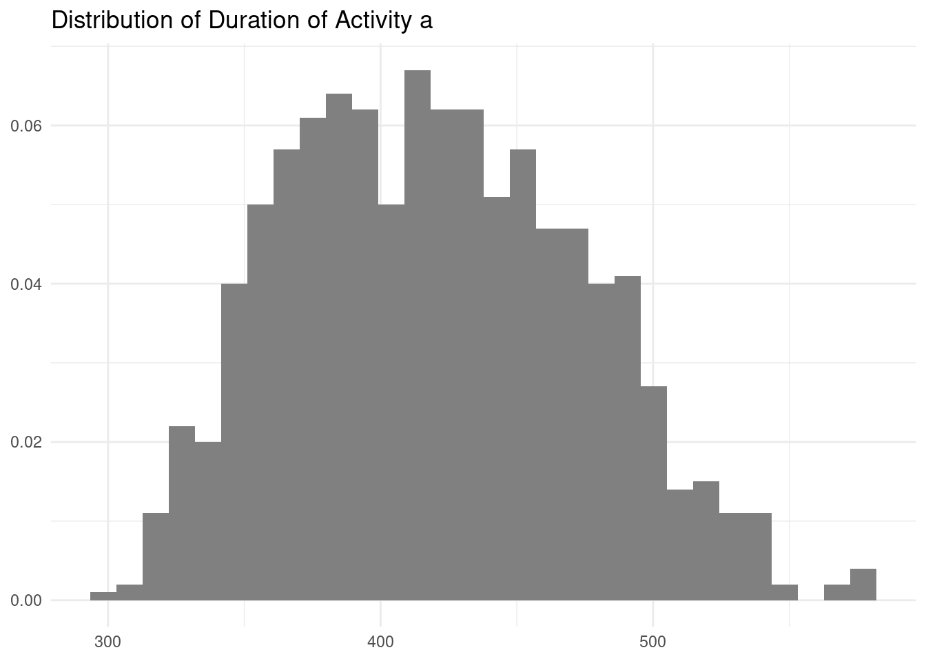
act_times[[1]]## [1] 441.1361 625.7911 500.3207 452.6212 437.1953 896.9015Let’s see the histogram of values of duration of activity a:
tibble(act_1 = map_dbl(act_times, ~ .[1])) |>
  ggplot(aes(act_1)) +
  geom_histogram(aes(y = after_stat(count / sum(count))), fill = "#808080") +
  theme_minimal() +
  labs(title = "Distribution of Duration of Activity a", x = NULL, y = NULL)
The values of the histogram lie between 300 and 600, the minimum and maximum value of duration of this activity.
To evaluate the project for each set of activity durations, I have defined the pert_eval() function. This function returns the expected time exp_time and the critical path cp.
pert_eval <- function(times){

  obj <- c(0, 0, 0, 1)
  mat <- matrix(c(1, 0, 0, 0,
                  -1, 0, 1, 0,
                  0, 1, 0, 0,
                  0, -1, 1, 0,
                  0, 0, -1, 1,
                  0, -1, 0, 1), nrow = 6, byrow = TRUE)
  dir <- rep(">=", 6)
  rhs <- times
  max <- FALSE

  sol <- Rglpk_solve_LP(obj = obj, mat = mat,
                        dir = dir, rhs = rhs, max = max)

  return(list(exp_time = sol$optimum,
              cp = sol$auxiliary$dual))

}
The evaluation of the first set of activity duration returns:
pert_eval(act_times[[1]])## $exp_time
## [1] 1504.123
##
## $cp
## [1] 1 1 0 0 1 0I am using again purrr:map() to evaluate pert_eval() for all values of act_times. The output is stored as a list of lists in act_times_eval.
set.seed(1111)
act_times_eval <- map(act_times, pert_eval)
Let’s extract the expected times and store them in the exp_times vector.
exp_times <- map_dbl(act_times_eval, ~ .$exp_time)To extract the critical path, first I put all values in a vector using purr::list_c(). Then I create the critical_paths data frame with the result and the activity names.
critical_paths <- tibble(activity = rep(letters[1:6], trials),
                         cp = map(act_times_eval, ~ .$cp) |> list_c())
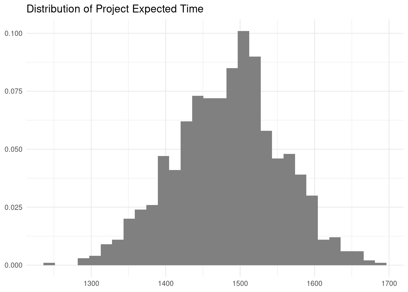
Let’s examine the properties of the expected time. It is now a probability distribution, of which we can examine the quantiles:
quantile(exp_times, seq(0, 1, 0.1))## 0% 10% 20% 30% 40% 50% 60% 70%
## 1246.257 1389.892 1422.152 1445.086 1467.629 1487.587 1504.957 1519.440
## 80% 90% 100%
## 1543.374 1576.341 1691.481From this result, we can make statements like estimating that 20% of times project time will be longer than 1543.37.
It can also be useful to plot the probability distribution of expected times.
tibble(et = exp_times) |>
  ggplot(aes(et)) +
  geom_histogram(aes(y = after_stat(count / sum(count))), fill = "#808080") +
  theme_minimal() +
  labs(title = "Distribution of Project Expected Time", x = NULL, y = NULL)
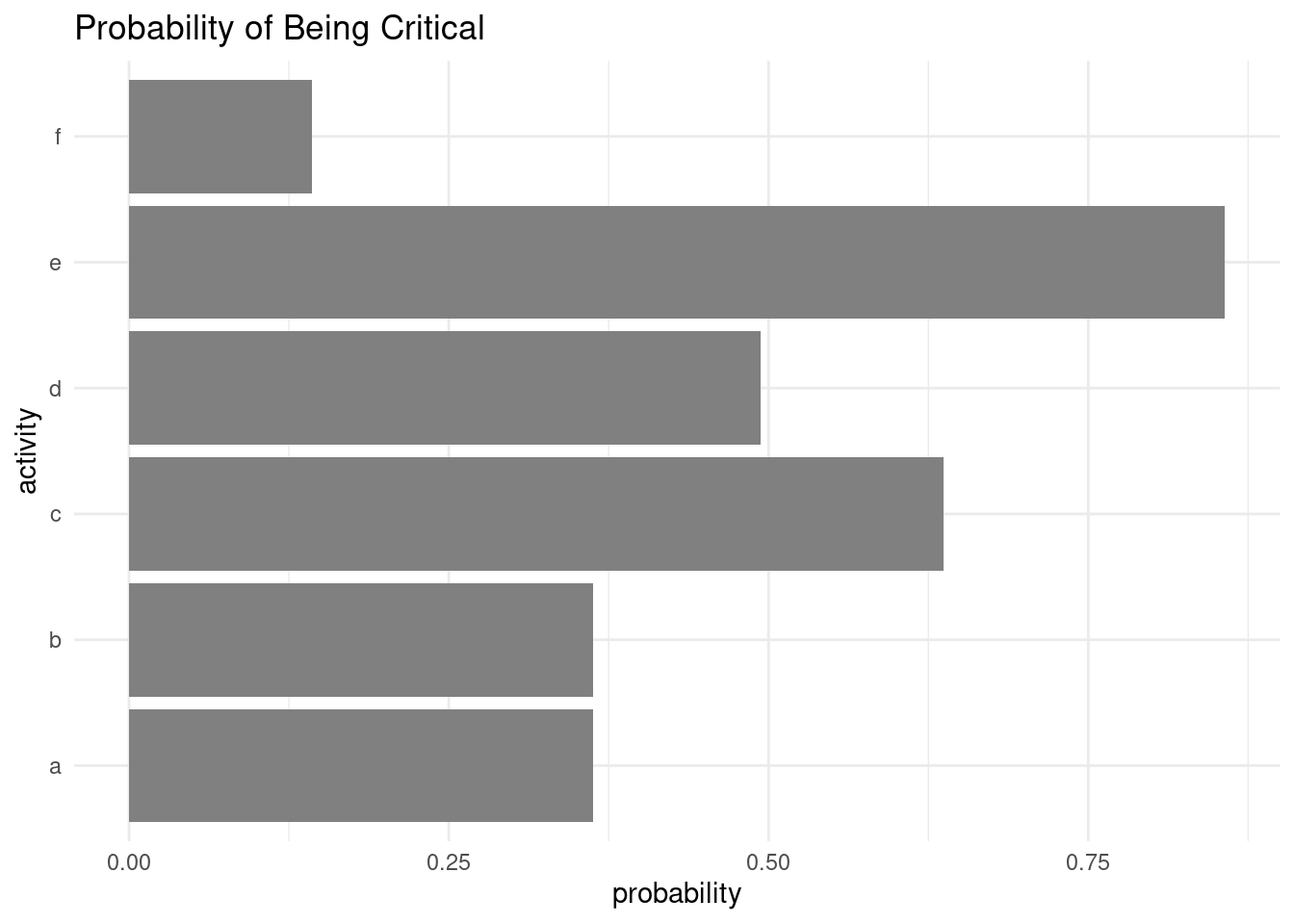
Respect to the critical path, we can examine how often each activity will be part of the critical path.
critical_paths |>
  filter(cp == 1) |>
  group_by(activity) |>
  summarise(freq = sum(cp)/trials) |>
  ggplot(aes(freq, activity)) +
  geom_col(fill = "#808080") +
  theme_minimal() +
  labs(title = "Probability of Being Critical", x = "probability", y = "activity")
The activity most likely of being critical is activity e, although in this case any activity can be critical depending on actual duration of the set of activities.
References:
- PERT probability distribution: https://jmsallan.netlify.app/blog/triangular-and-pert-probability-distributions/
- Monte Carlo simulation: https://jmsallan.netlify.app/blog/2024-10-04-analyzing-a-lottery-with-monte-carlo-simulation/
Session Info
## R version 4.4.2 (2024-10-31)
## Platform: x86_64-pc-linux-gnu
## Running under: Linux Mint 21.1
##
## Matrix products: default
## BLAS:   /usr/lib/x86_64-linux-gnu/blas/libblas.so.3.10.0
## LAPACK: /usr/lib/x86_64-linux-gnu/lapack/liblapack.so.3.10.0
##
## locale:
##  [1] LC_CTYPE=es_ES.UTF-8       LC_NUMERIC=C
##  [3] LC_TIME=es_ES.UTF-8        LC_COLLATE=es_ES.UTF-8
##  [5] LC_MONETARY=es_ES.UTF-8    LC_MESSAGES=es_ES.UTF-8
##  [7] LC_PAPER=es_ES.UTF-8       LC_NAME=C
##  [9] LC_ADDRESS=C               LC_TELEPHONE=C
## [11] LC_MEASUREMENT=es_ES.UTF-8 LC_IDENTIFICATION=C
##
## time zone: Europe/Madrid
## tzcode source: system (glibc)
##
## attached base packages:
## [1] stats     graphics  grDevices utils     datasets  methods   base
##
## other attached packages:
##  [1] igraph_2.0.3     mc2d_0.2.1       mvtnorm_1.2-5    Rglpk_0.6-4
##  [5] slam_0.1-50      kableExtra_1.4.0 lubridate_1.9.3  forcats_1.0.0
##  [9] stringr_1.5.1    dplyr_1.1.4      purrr_1.0.2      readr_2.1.5
## [13] tidyr_1.3.1      tibble_3.2.1     ggplot2_3.5.1    tidyverse_2.0.0
##
## loaded via a namespace (and not attached):
##  [1] gtable_0.3.5      xfun_0.43         bslib_0.7.0       rstatix_0.7.2
##  [5] tzdb_0.4.0        vctrs_0.6.5       tools_4.4.2       generics_0.1.3
##  [9] fansi_1.0.6       highr_0.10        pkgconfig_2.0.3   lifecycle_1.0.4
## [13] compiler_4.4.2    farver_2.1.1      munsell_0.5.1     carData_3.0-5
## [17] htmltools_0.5.8.1 sass_0.4.9        yaml_2.3.8        pillar_1.9.0
## [21] car_3.1-2         ggpubr_0.6.0      jquerylib_0.1.4   cachem_1.0.8
## [25] abind_1.4-5       tidyselect_1.2.1  digest_0.6.35     stringi_1.8.3
## [29] bookdown_0.39     labeling_0.4.3    fastmap_1.1.1     grid_4.4.2
## [33] colorspace_2.1-0  cli_3.6.2         magrittr_2.0.3    utf8_1.2.4
## [37] broom_1.0.5       withr_3.0.0       scales_1.3.0      backports_1.4.1
## [41] timechange_0.3.0  rmarkdown_2.26    ggsignif_0.6.4    blogdown_1.19
## [45] hms_1.1.3         evaluate_0.23     knitr_1.46        viridisLite_0.4.2
## [49] rlang_1.1.3       glue_1.7.0        xml2_1.3.6        svglite_2.1.3
## [53] rstudioapi_0.16.0 jsonlite_1.8.8    R6_2.5.1          systemfonts_1.0.6