R packages are bundles of code, data, documentation and test structured to be easily shared through repositories like CRAN. An R package usually needs other packages to work, or maybe needs some other packages for optional functionalities. There are three ways of specifying these dependencies in the DESCRIPTION file of a package:
- Prior to the roll-out of namespaces in R 2.14.0 in 2011,
Dependswas the only way to establish that the package depends on another package. Nowadays, dependencies are listed inImports. We can useDependsto state a minimum version for R itself, e.g.Depends: R (>= 3.6.0). - Packages listed in
Importsare needed by package users at runtime. Any time the package is installed, those packages will also be installed, if not already present. - Packages listed in
Suggestsare either needed for development tasks or might unlock optional functionalities. They are not automatically installed along with the package.
The relationship dependencies between a set of R packages leads to the definition of a directed network of dependencies, where nodes are packages connected through a direct link (i,j) if package j has some dependency on package i.
To explore how these networks of dependencies look like, I will examine the network of packages installed in my computer. I will use tidygraph and ggraph for graph manipulation and plotting, and data.table and dplyr for tabular data handling.
library(data.table)
library(dplyr)
library(tidygraph)
library(ggraph)
library(patchwork)
library(kableExtra)
I have checked the packages installed in my computer using installed.packages(). The output is a matrix, that I transform to a data.table object. This list of packages will be different for every R user, and will be representative of its preferences and of how he or she is using R.
ip <- data.table(installed.packages())Dependencies are listed in the Depends, Imports and Suggests columns. Let’s see the Depends column:
ip[, .(Package, Depends)]## Package Depends
## 1: abind R (>= 1.5.0)
## 2: arm R (>= 3.1.0), MASS, Matrix (>= 1.0), stats, lme4 (>= 1.0)
## 3: askpass <NA>
## 4: assertthat <NA>
## 5: backports R (>= 3.0.0)
## ---
## 310: stats4 <NA>
## 311: survival R (>= 3.5.0)
## 312: tcltk <NA>
## 313: tools <NA>
## 314: utils <NA>I am building a table of dependencies with the get_table_packages() function:
- Selects a specific
columnof dependencies. - gets each of the packages of each row in the column with
data:table::tstrsplit. - Transforms the values of each package so that it represents a package name only. For instance,
dplyr (>= 0.8.5)is transformed intodplyrandR (>= 2.10.0)intoR. - Pivots the table into a long table with
originanddestinationcolumns. - Adds a
relationcolumn to store all data in a single table.
get_table_packages <- function(dt, column){

  table <- copy(dt)
  vars <- c("Package", column)

  table <- table[, ..vars]

  table <- cbind(table[, 1], table[ , tstrsplit(table[[2]], ",")])
  table <- table[, lapply(.SD, \(x) gsub("^ ", "", x))]
  table <- table[, lapply(.SD, \(x) gsub(">=", " ", x))]
  table <- table[, lapply(.SD, \(x) gsub("\n", "", x))]
  table <- table[, lapply(.SD, \(x) gsub("\\(", "", x))]
  table <- table[, lapply(.SD, \(x) sapply(strsplit(x, " "), \(x) x[1]))]
  table <- melt(table, id.vars = "Package", na.rm = TRUE)

  table[, variable := NULL]
  table[, relation := column]
  setnames(table, c("destination", "origin", "relation"))
  setcolorder(table, c("origin", "destination", "relation"))

  return(table)

}
Finally I am applying the function to each dependency and storing the results in ip_table.
rel_packages <- c("Depends", "Imports", "Suggests")

ip_list <- lapply(rel_packages, \(x) get_table_packages(ip, x))

ip_table <- rbindlist(ip_list)

rm(ip_list)
Obtaining package networks
Let’s obtain the three dependency networks defined in rel_packages and store then in a list. I am also calculating three node measures:
- in-degree
d_in, the number of edges incident to a node. - out-degree
d_out, the number of edges going out of a node. - betweenness
btw, the number of shortest paths passing through a node.
network_packages <- lapply(rel_packages, function(x){

  g <- tbl_graph(edges = ip_table[relation == x], directed = TRUE)

  g <- g %>%
    activate(nodes) %>%
    mutate(d_in = centrality_degree(mode = "in"),
         d_out = centrality_degree(mode = "out"),
         btw = centrality_betweenness())

  return(g)
})

names(network_packages) <- rel_packages
Let’s examine each of the produced networks.
network_packages## $Depends
## # A tbl_graph: 232 nodes and 306 edges
## #
## # A directed acyclic simple graph with 1 component
## #
## # Node Data: 232 × 4 (active)
## name d_in d_out btw
## <chr> <dbl> <dbl> <dbl>
## 1 R 0 215 0
## 2 abind 1 0 0
## 3 arm 5 0 0
## 4 backports 1 0 0
## 5 BAdatasets 1 0 0
## 6 BAdatasetsSpatial 1 0 0
## # … with 226 more rows
## #
## # Edge Data: 306 × 3
## from to relation
## <int> <int> <chr>
## 1 1 2 Depends
## 2 1 3 Depends
## 3 1 4 Depends
## # … with 303 more rows
##
## $Imports
## # A tbl_graph: 299 nodes and 1359 edges
## #
## # A directed acyclic simple graph with 1 component
## #
## # Node Data: 299 × 4 (active)
## name d_in d_out btw
## <chr> <dbl> <dbl> <dbl>
## 1 methods 2 62 191.
## 2 abind 2 2 0.167
## 3 arm 7 1 18
## 4 sys 0 3 0
## 5 askpass 1 3 13
## 6 tools 0 20 0
## # … with 293 more rows
## #
## # Edge Data: 1,359 × 3
## from to relation
## <int> <int> <chr>
## 1 1 2 Imports
## 2 2 3 Imports
## 3 4 5 Imports
## # … with 1,356 more rows
##
## $Suggests
## # A tbl_graph: 669 nodes and 1987 edges
## #
## # A directed simple graph with 5 components
## #
## # Node Data: 669 × 4 (active)
## name d_in d_out btw
## <chr> <dbl> <dbl> <dbl>
## 1 testthat 11 175 20816.
## 2 askpass 1 0 0
## 3 assertthat 2 1 0.5
## 4 BBmisc 3 0 0
## 5 bit 7 1 294.
## 6 covr 0 109 0
## # … with 663 more rows
## #
## # Edge Data: 1,987 × 3
## from to relation
## <int> <int> <chr>
## 1 1 2 Suggests
## 2 1 3 Suggests
## 3 1 4 Suggests
## # … with 1,984 more rowsWe observe that:
- The networks of
DependsandImportsare trees. This makes sense since there may not be cyclical dependencies or imports. The set of nodes of both networks is a subset of the installed packages. - The network of
Suggestshas cycles. The set of nodes is larger than the one of installed packages, indicating that some suggested packages are not installed.
Plotting the networks
I am defining a plot_network_packages function to plot the networks. Note how I am choosing a very low value of transparency alpha for edges, as networks are relatively dense.
plot_network_packages <- function(i){
  ggraph(network_packages[[i]], layout = "sugiyama") +
  geom_node_point(aes(label = name)) +
  geom_edge_link(alpha = 0.1, start_cap = circle(3, 'mm'), end_cap = circle(3, 'mm'), arrow = arrow(length = unit(2, 'mm'))) +
  theme_graph() +
  labs(title = paste("Network of", names(network_packages)[i]))
}

network_plots <- lapply(1:3, plot_network_packages)
To plot all networks at once, I am using wrap_plots from the patchwork package. Functions from gridExtra do not seem to work well with ggraph outcomes.
wrap_plots(network_plots, ncol = 1)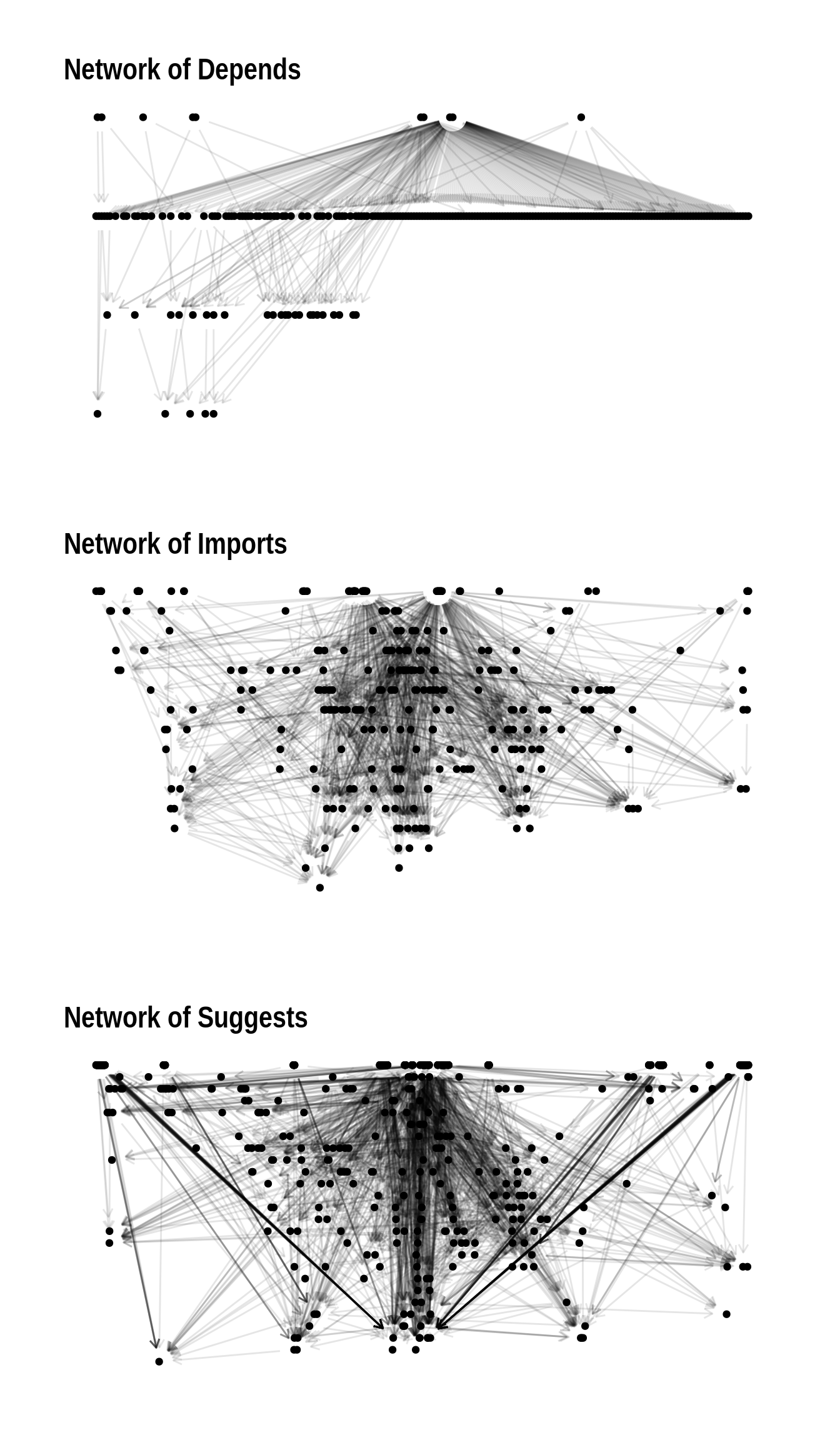
We observe that Depends and Imports have a tree like structure, more complex for Imports. Although the Suggests network has cycles and disconnected components, seems to behave like a tree for most of its nodes.
Relevant nodes
Seeing that the networks of packages have a tree-like structure, we can establish two criteria to select relevant nodes:
- Root nodes: the packages at the top of the tree seem to be critical for the functionality of the system. Root nodes will have in-degree equal to zero, and high values of out degree.
- Intermediate nodes: for paths of relationships of two or more edges, the nodes in the middle are also important for package functionality. These nodes will have high values of betweenness.
Let’s create a function to present the relevant packages of a network.
get_table_measure <- function(i, nnodes = 5){

  node_table <- network_packages[[i]] %>%
    activate(nodes) %>%
    as_tibble()

  root <- node_table %>%
    filter(d_in == 0) %>%
    arrange(-d_out) %>%
    mutate(relation = names(network_packages)[i]) %>%
    select(relation, name, d_out) %>%
    rename(root = name) %>%
    slice(1:nnodes)

  interm <- node_table %>%
    arrange(-btw) %>%
    select(name, btw) %>%
    rename(intermediate = name) %>%
    slice(1:nnodes)

  table <- bind_cols(root, interm)

  return(table)

}
Here is the result of applying the function, presented in a table formatted with kableExtra.
nodes_list <- lapply(1:3, \(i) get_table_measure(i))
nodes_table <- bind_rows(nodes_list)

nodes_table %>%
  kbl() %>%
  kable_paper(full_width = FALSE) %>%
  row_spec(1:5, background = "#FFFFCC") %>%
   row_spec(6:10, background = "#CCFFFF") %>%
row_spec(11:15, background = "#FFCCCC")| relation | root | d_out | intermediate | btw |
|---|---|---|---|---|
| Depends | R | 215 | MASS | 7.000000 |
| Depends | methods | 16 | doParallel | 3.333333 |
| Depends | stats | 15 | rpart | 3.000000 |
| Depends | utils | 11 | mlr | 1.333333 |
| Depends | graphics | 6 | Formula | 1.250000 |
| Imports | utils | 96 | ggplot2 | 326.386325 |
| Imports | grDevices | 38 | tibble | 323.841281 |
| Imports | magrittr | 30 | stats | 197.158883 |
| Imports | tools | 20 | methods | 190.992857 |
| Imports | R6 | 20 | scales | 146.116667 |
| Suggests | covr | 109 | broom | 29349.582022 |
| Suggests | spelling | 22 | dplyr | 28755.545378 |
| Suggests | mockery | 12 | testthat | 20815.623867 |
| Suggests | codetools | 10 | knitr | 20242.894993 |
| Suggests | survival | 10 | ggplot2 | 17459.763665 |
Root and intermediate packages are different for each network, representative of each relationship. The main root package in Depends is the minimal version of R required. This was to be expected, given the role of Depends on package dependencies definition. Root packages in Imports are related with the tidyverse like magrittr or with data visualization like grDevices. Root packages in Suggests are related with package development, and most of them are not installed in my computer.
As for intermediate packages, the ones in Depends are not quite representative, as this relationship is not intended to be chained at several levels. The results of Imports are more informative, and show the relevance of the tidyverse in package development, at least the ones in my computer. This is also evident in Suggests, where together with package development appear other packages related with publishing and visualization like knitr and ggplot2.
The results of this analysis are not representative of the whole R CRAN package ecosystem. They have to be considered as a preliminary analysis for a further examination of the whole CRAN network.
References
- Depends or imports? (From the Developing R packages course) https://campus.datacamp.com/courses/developing-r-packages/checking-and-building-r-packages?ex=8
- Dependencies: What does your package need? (from Wickham, H. & Bryant, J. R packages) https://r-pkgs.org/description.html#description-dependencies
Session info
## R version 4.2.0 (2022-04-22)
## Platform: x86_64-pc-linux-gnu (64-bit)
## Running under: Linux Mint 19.2
##
## Matrix products: default
## BLAS:   /usr/lib/x86_64-linux-gnu/openblas/libblas.so.3
## LAPACK: /usr/lib/x86_64-linux-gnu/libopenblasp-r0.2.20.so
##
## locale:
##  [1] LC_CTYPE=es_ES.UTF-8       LC_NUMERIC=C
##  [3] LC_TIME=es_ES.UTF-8        LC_COLLATE=es_ES.UTF-8
##  [5] LC_MONETARY=es_ES.UTF-8    LC_MESSAGES=es_ES.UTF-8
##  [7] LC_PAPER=es_ES.UTF-8       LC_NAME=C
##  [9] LC_ADDRESS=C               LC_TELEPHONE=C
## [11] LC_MEASUREMENT=es_ES.UTF-8 LC_IDENTIFICATION=C
##
## attached base packages:
## [1] stats     graphics  grDevices utils     datasets  methods   base
##
## other attached packages:
## [1] kableExtra_1.3.4  patchwork_1.1.1   ggraph_2.0.5      ggplot2_3.3.5
## [5] tidygraph_1.2.1   dplyr_1.0.9       data.table_1.14.2
##
## loaded via a namespace (and not attached):
##  [1] tidyselect_1.1.2   xfun_0.30          bslib_0.3.1        purrr_0.3.4
##  [5] graphlayouts_0.8.0 colorspace_2.0-3   vctrs_0.4.1        generics_0.1.2
##  [9] viridisLite_0.4.0  htmltools_0.5.2    yaml_2.3.5         utf8_1.2.2
## [13] rlang_1.0.2        jquerylib_0.1.4    pillar_1.7.0       glue_1.6.2
## [17] withr_2.5.0        DBI_1.1.2          tweenr_1.0.2       lifecycle_1.0.1
## [21] stringr_1.4.0      munsell_0.5.0      blogdown_1.9       gtable_0.3.0
## [25] rvest_1.0.2        evaluate_0.15      labeling_0.4.2     knitr_1.39
## [29] fastmap_1.1.0      fansi_1.0.3        highr_0.9          Rcpp_1.0.8.3
## [33] scales_1.2.0       webshot_0.5.3      jsonlite_1.8.0     systemfonts_1.0.4
## [37] farver_2.1.0       gridExtra_2.3      ggforce_0.3.3      digest_0.6.29
## [41] stringi_1.7.6      bookdown_0.26      ggrepel_0.9.1      polyclip_1.10-0
## [45] grid_4.2.0         cli_3.3.0          tools_4.2.0        magrittr_2.0.3
## [49] sass_0.4.1         tibble_3.1.6       crayon_1.5.1       tidyr_1.2.0
## [53] pkgconfig_2.0.3    ellipsis_0.3.2     MASS_7.3-57        xml2_1.3.3
## [57] svglite_2.1.0      httr_1.4.2         viridis_0.6.2      assertthat_0.2.1
## [61] rmarkdown_2.14     rstudioapi_0.13    R6_2.5.1           igraph_1.3.1
## [65] compiler_4.2.0