Dense visualization in R with ggrepel and plotly

Jose M Sallan 2022-05-02 14 min read

Sometimes we need to visualize datasets with many information and it is hard to set all the information at the same time. It may be the case of scatterplots with many points of which we need to present node labels. In this post I will present two possible solutions for this problem:

Resetting labels with package ggrepel.
Doing interactive plots with plotly.

In addition to this two packages, I will be using dplyr for data handling, ggplot2 for plotting and zoo to calculate rolling means.

library(dplyr)
library(ggplot2)
library(ggrepel)
library(plotly)
library(zoo)

Let’s use the txhousing dataset to plot the values of median and sales for Texas cities in a specific month. I have set nudge_y = 4000 to separate text from point.

txhousing %>%
  filter(year == 2005, month == 7) %>%
  filter(!is.na(sales), !is.na(median)) %>%
  ggplot(aes(sales, median, label = city)) +
  geom_point() +
  geom_text(nudge_y = 4000, size = 3) +
  scale_x_log10() +
  theme_minimal()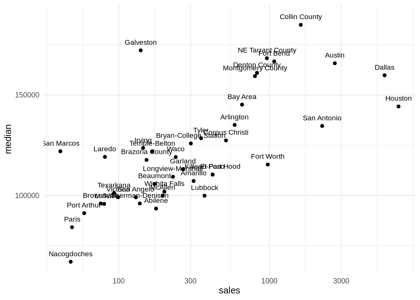

Although I have reduced somewhat the size of labels and adjusted sales logarithmically, there is still a huge overlay of labels.

Using ggrepel

The ggrepel provides geoms for ggplot2 to repel overlapping text labels:

geom_text_repel()
geom_label_repel()

After loading the package, we only need to replace geom_text() with geom_text_repel(). Now we can override the nudge_y argument as the package detachs the text from the point.

txhousing %>%
  filter(year == 2005, month == 7) %>%
  filter(!is.na(sales), !is.na(median)) %>%
  ggplot(aes(sales, median, label = city)) +
  geom_point() +
  geom_text_repel(size = 3) +
  scale_x_log10() +
  theme_minimal()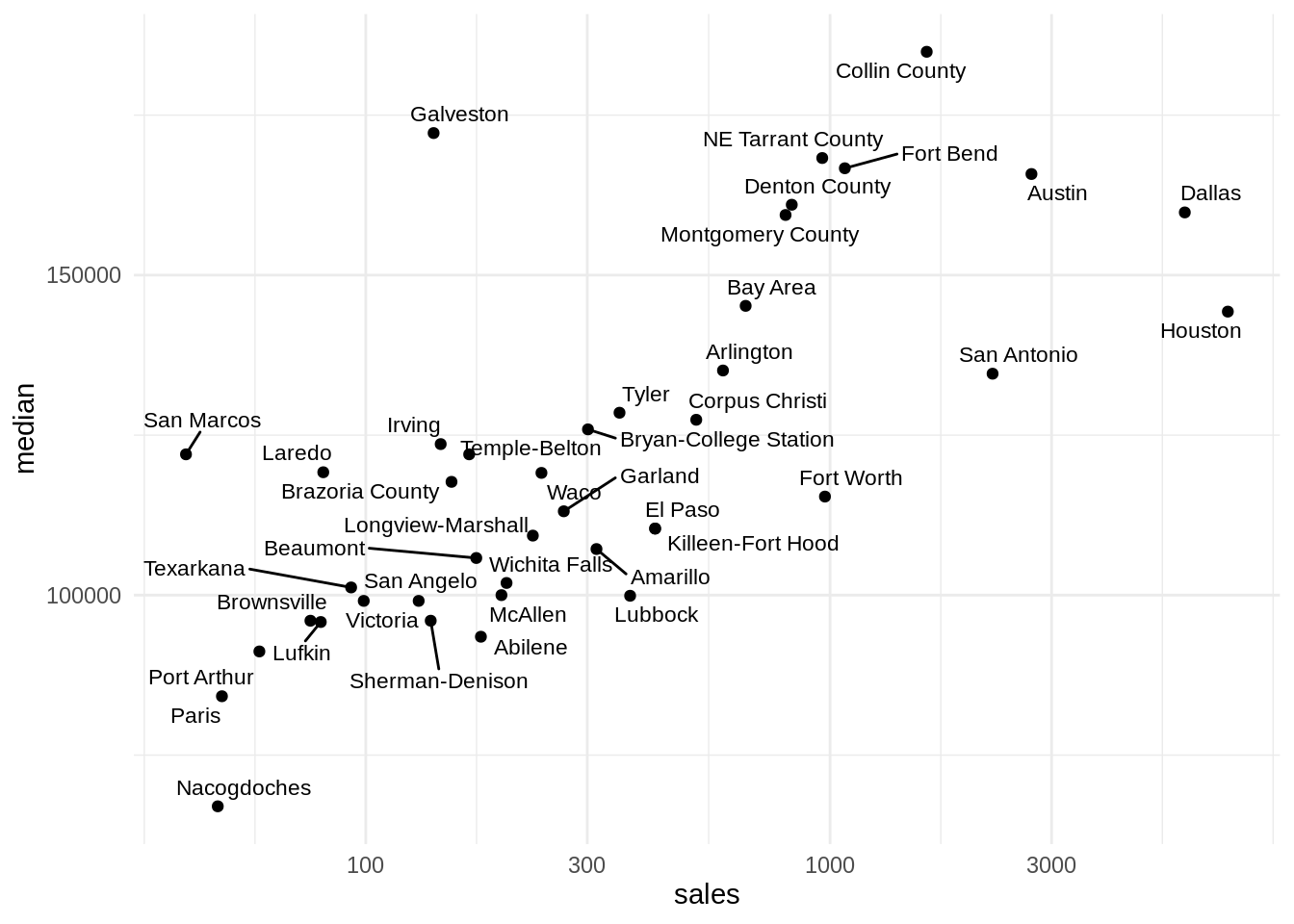

Using plotly

Another possibility to present labels is to create an interactive plot with plotly, an R package for creating interactive web-based graphs via the open source JavaScript graphing library plotly.js. These graphics can be made interactive in a html setting, like a Shiny app or a rnmarkdown document. You only need to set the cursor over the point to see a label (tooltip) with the name of the city on it.

Steps to do the plot:

Set the content of the label to present (tooltip) in the text parameter of aes.
Save the plot in a variable.
Present the plot using the ggplotly function with tooltip = "text".

tx_ply <- txhousing %>%
  filter(year == 2005, month == 7) %>%
  filter(!is.na(sales), !is.na(median)) %>%
  ggplot(aes(sales, median, text = city)) +
  geom_point() +
  scale_x_log10() +
  theme_minimal()

ggplotly(tx_ply, tooltip = "text")

Here is an example of a more complex tooltip.

tx_ply2 <- txhousing %>%
  filter(year == 2005, month == 7) %>%
  filter(!is.na(sales), !is.na(median)) %>%
  ggplot(aes(sales, median, 
             text = paste("City: ", city, "\n",
                         "Median:", median, "\n",
                         "Sales:", sales))) +
  geom_point() +
  scale_x_log10() +
  theme_minimal()
  
ggplotly(tx_ply2, tooltip = "text")

A line plot with plotly

Let’s see the rolling mean of the evolution of sales of the largest Texan cities:

txhousing %>%
  filter(city %in% c("Houston", "Dallas")) %>%
  group_by(city) %>%
  mutate(av_sales = rollmean(sales, k = 12, fill = NA, na.rm = TRUE)) %>%
  ungroup() %>%
  filter(!is.na(av_sales)) %>%
  select(date, city, av_sales) %>%
  ggplot(aes(date, av_sales, color = city)) +
  geom_line() +
  theme_minimal() +
  theme(legend.position = c(0.1, 0.8)) +
  labs(x = "date", y = "sales", title = "Sales in large Texas cities")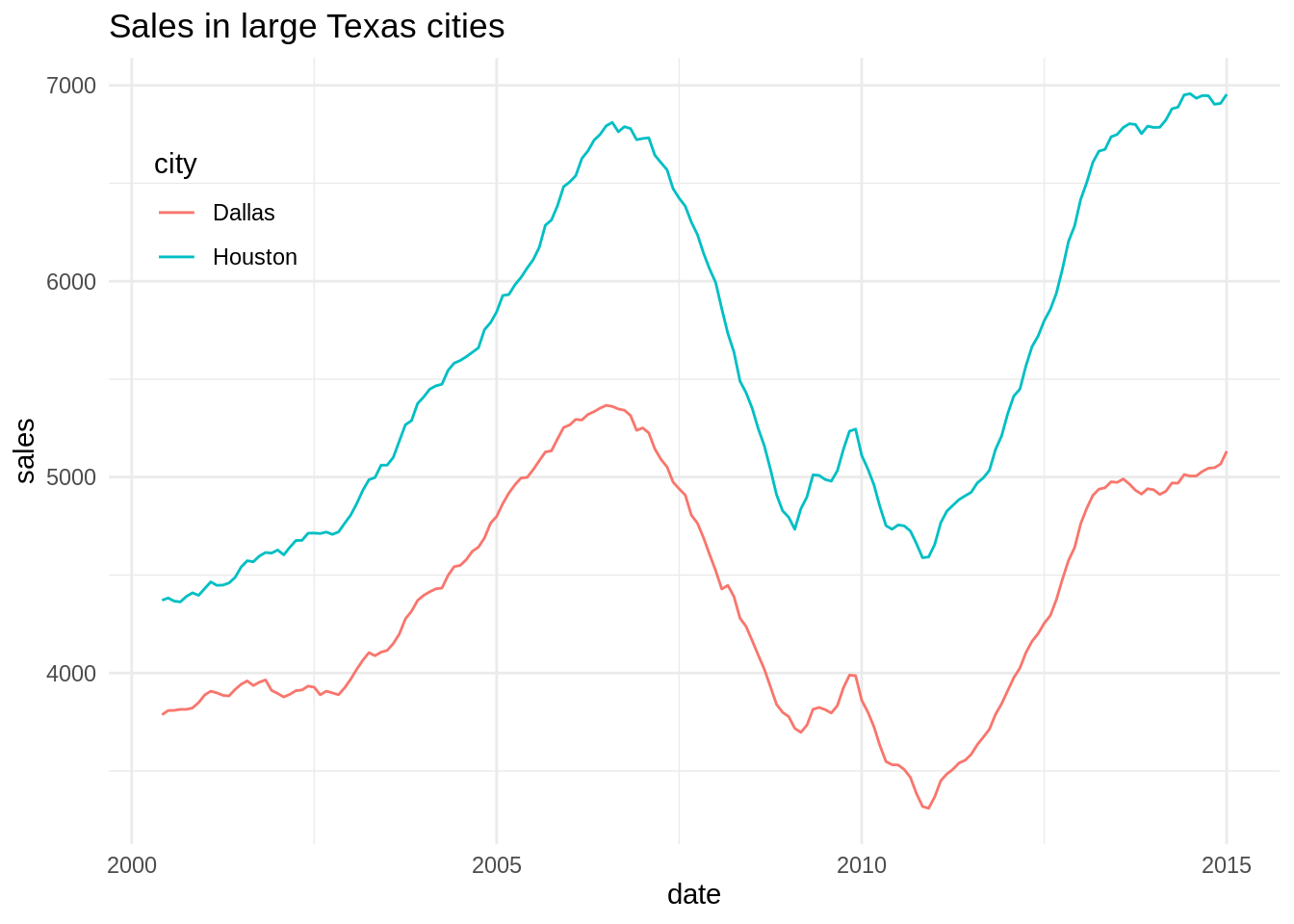

Here is the same plot with plotly. Note that I have removed the legend as it is not necessary in this context. If you hover one of the lines you will see the starndard tooltip.

tx_line <- txhousing %>%
  filter(city %in% c("Houston", "Dallas")) %>%
  group_by(city) %>%
  mutate(av_sales = rollmean(sales, k = 12, fill = NA, na.rm = TRUE)) %>%
  ungroup() %>%
  filter(!is.na(av_sales)) %>%
  select(date, city, av_sales) %>%
  ggplot(aes(date, av_sales, color = city)) +
  geom_line() +
  theme_minimal() +
  theme(legend.position = "none") +
  labs(x = "date", y = "sales", title = "Sales in large Texas cities")

ggplotly(tx_line)

Using ggrepel and plotly

We can use ggrepel and plotly to present visualizations with dense information. While ggrepel can be adequate for printed or PDF outcomes, plotly offers the possibility of presenting interactive plots in html format.

References

Getting started with plotly in ggplot2 https://plotly.com/ggplot2/getting-started/
Fitton, Daniel (2018). Plotly in R: How to make ggplot2 charts interactive with ggplotly. https://www.musgraveanalytics.com/blog/2018/8/24/how-to-make-ggplot2-charts-interactive-with-plotly
Slowikowski, Kamil (2021-01-15). Getting started with ggrepel. https://cran.r-project.org/web/packages/ggrepel/vignettes/ggrepel.html

Session info

## R version 4.2.0 (2022-04-22)
## Platform: x86_64-pc-linux-gnu (64-bit)
## Running under: Linux Mint 19.2
## 
## Matrix products: default
## BLAS:   /usr/lib/x86_64-linux-gnu/openblas/libblas.so.3
## LAPACK: /usr/lib/x86_64-linux-gnu/libopenblasp-r0.2.20.so
## 
## locale:
##  [1] LC_CTYPE=es_ES.UTF-8       LC_NUMERIC=C              
##  [3] LC_TIME=es_ES.UTF-8        LC_COLLATE=es_ES.UTF-8    
##  [5] LC_MONETARY=es_ES.UTF-8    LC_MESSAGES=es_ES.UTF-8   
##  [7] LC_PAPER=es_ES.UTF-8       LC_NAME=C                 
##  [9] LC_ADDRESS=C               LC_TELEPHONE=C            
## [11] LC_MEASUREMENT=es_ES.UTF-8 LC_IDENTIFICATION=C       
## 
## attached base packages:
## [1] stats     graphics  grDevices utils     datasets  methods   base     
## 
## other attached packages:
## [1] zoo_1.8-10    plotly_4.10.0 ggrepel_0.9.1 ggplot2_3.3.5 dplyr_1.0.9  
## 
## loaded via a namespace (and not attached):
##  [1] tidyselect_1.1.2  xfun_0.30         bslib_0.3.1       purrr_0.3.4      
##  [5] lattice_0.20-45   colorspace_2.0-3  vctrs_0.4.1       generics_0.1.2   
##  [9] htmltools_0.5.2   viridisLite_0.4.0 yaml_2.3.5        utf8_1.2.2       
## [13] rlang_1.0.2       jquerylib_0.1.4   pillar_1.7.0      glue_1.6.2       
## [17] withr_2.5.0       DBI_1.1.2         lifecycle_1.0.1   stringr_1.4.0    
## [21] munsell_0.5.0     blogdown_1.9      gtable_0.3.0      htmlwidgets_1.5.4
## [25] evaluate_0.15     labeling_0.4.2    knitr_1.39        fastmap_1.1.0    
## [29] crosstalk_1.2.0   fansi_1.0.3       highr_0.9         Rcpp_1.0.8.3     
## [33] scales_1.2.0      jsonlite_1.8.0    farver_2.1.0      digest_0.6.29    
## [37] stringi_1.7.6     bookdown_0.26     grid_4.2.0        cli_3.3.0        
## [41] tools_4.2.0       magrittr_2.0.3    sass_0.4.1        lazyeval_0.2.2   
## [45] tibble_3.1.6      crayon_1.5.1      tidyr_1.2.0       pkgconfig_2.0.3  
## [49] ellipsis_0.3.2    data.table_1.14.2 assertthat_0.2.1  rmarkdown_2.14   
## [53] httr_1.4.2        rstudioapi_0.13   R6_2.5.1          compiler_4.2.0

The Jose M Sallan static website