When we build predictive models for time series, forecasting consists of predicting values of the future with values of the past or present. Therefore, the strategies of cross validation are different from cross sectional datasets.
In this post, I will present three cross validation strategies for time series: stretching windows, sliding windows and tiling windows. Then, I will show how to implement these strategies with the tidyverts family of packages:
library(tidyverse)

library(tsibble)
library(feasts)
library(fable)
Stretching Windows
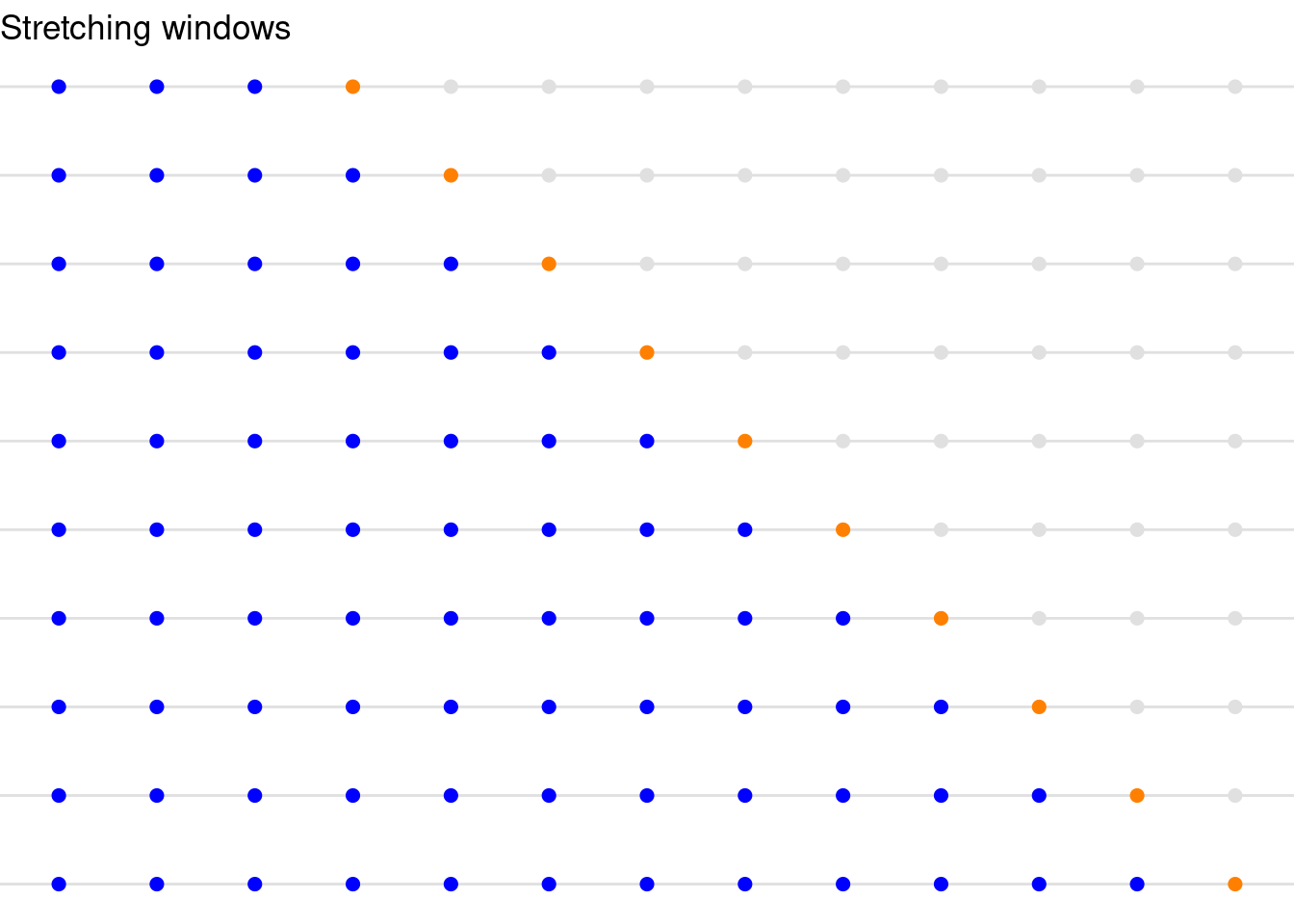
Stretching windows (also called expanding windows) begin with a smaller window and then expand over time, gradually including more of the past data points. With each step forward, the window size increases, covering all the data points from the start to the current point.
Stretching windows are useful when you want to incorporate all available historical data up to a certain point for modeling. The idea is to use all the past information to predict the future as time progresses. It can be useful for cumulative modelling in time series, where each additional data point is important to forecast the time series.
n_y <- 10
s_x <- 3 # for stretching windows
n_x <- n_y + s_x

grid_stretch <- expand_grid(x = 1:n_x, y = 1:n_y)

grid_stretch <- grid_stretch |>
  mutate(stretch = case_when(
    x <= n_y + s_x - y ~ "stretch",
    x == n_y + s_x +1 -y ~ "test",
    TRUE ~ "future"
  ))

grid_stretch |>
  ggplot(aes(x, y, color = stretch)) +
  geom_hline(yintercept = 1:n_y, color = "#E0E0E0") +
  geom_point(size = 2) +
  theme_void() +
  theme(legend.position = "none") +
  scale_color_manual(values = c("#E0E0E0", "#0000FF", "#FF8000")) +
  ggtitle(label = "Stretching windows")
Sliding Windows
The sliding window method uses a fixed-size window that “slides” over the time series data. At each step, the window shifts by one or more time points, moving forward in time.
This method makes predictions so that each step captures the most recent observations. It is useful in context where temporal dependencies are critical, and observations too far in time are not useful for the prediction job.
n_x <- 15
s_w <- 5  # for sliding windows
n_y <- n_x


grid_slide <- expand_grid(x = 1:n_x, y = 1:n_y)

grid_slide <- grid_slide |>
  mutate(slide = case_when(x <= n_y - y & x >= n_y - s_w + 1 - y ~ "slide",
                           x == n_y + 1 - y ~ "test",
                           TRUE ~ "future"
  ))

grid_slide |>
  filter(y <= n_y - s_w) |>
  ggplot(aes(x, y, color = slide)) +
  geom_hline(yintercept = 1:(n_y - s_w), color = "#E0E0E0") +
  geom_point(size = 2) +
  theme_void() +
  theme(legend.position = "none") +
  scale_color_manual(values = c("#E0E0E0", "#0000FF", "#FF8000")) +
  ggtitle(label = "Sliding windows")
Tiling Windows
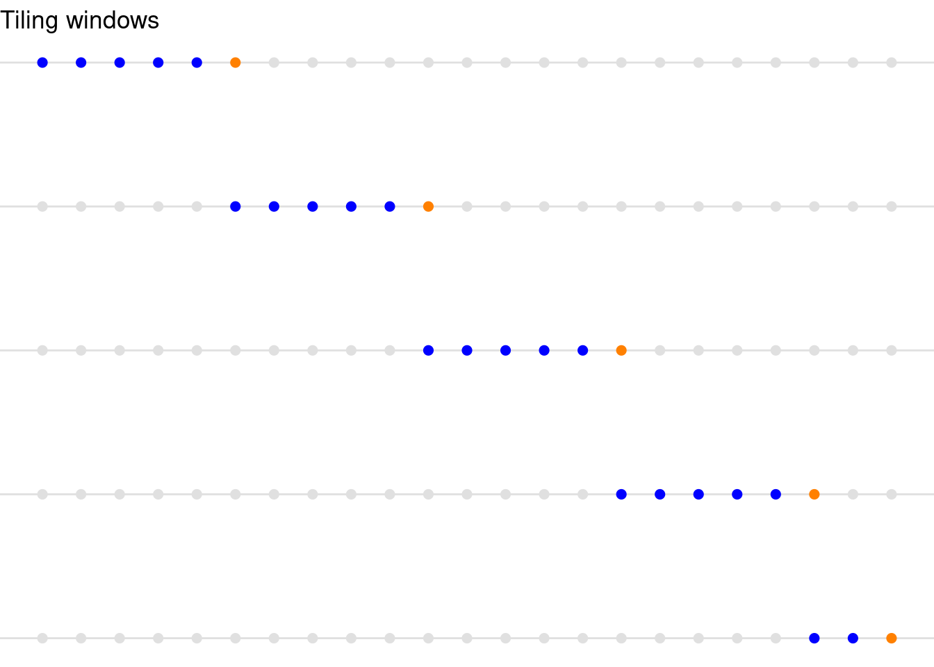
Tiling windows divide the time series into disjoint (non-overlapping) windows or segments. Each window contains a fixed number of consecutive data points, and once a window is processed, the next segment of data is used without overlap. This method can be suitable for situations where partitioning the time series into non-overlapping sections makes sense, like periodic tasks or batch processing where you’re analyzing discrete segments independently.
n_x <- 23
w_t <- 5  # for tiling windows
n_y <- floor(n_x/w_t) + 1

grid_tile <- expand_grid(x = 1:n_x, y = 1:n_y)

x_min <- c(w_t*(n_y-1):1 + 1, 1)
x_max <- c(n_x-1, w_t*(n_y-1):1)

bounds <- tibble(y = 1:n_y, x_min = x_min, x_max = x_max)

grid_tile <- grid_tile |>
  left_join(bounds, by = "y")

grid_tile <- grid_tile |>
  mutate(tile = case_when(x >= x_min & x <= x_max ~ "slide",
                           x == x_max + 1 ~ "test",
                           TRUE ~ "future"
  ))

grid_tile |>
  ggplot(aes(x, y, color = tile)) +
  geom_hline(yintercept = 1:n_y, color = "#E0E0E0") +
  geom_point(size = 2) +
  theme_void() +
  theme(legend.position = "none") +
  scale_color_manual(values = c("#E0E0E0", "#0000FF", "#FF8000")) +
  ggtitle(label = "Tiling windows")
Dataset tourism
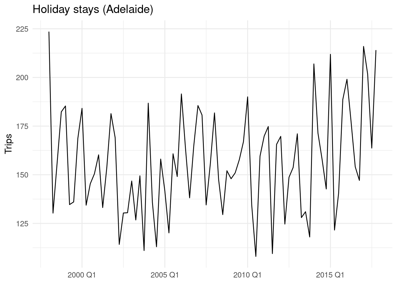
To illustrate how to perform cross validation with time series using the methods described above, I will use a subset of the tourism dataset, provided with the tsibble package. The adelaide_holiday time series include the number of holiday trips to Adelaide:
adelaide_holiday <- tourism |>
  filter(Region == "Adelaide", Purpose == "Holiday")
We can obtain a plot of the time series with autoplot().
adelaide_holiday |>
  autoplot(.vars = Trips) +
  theme_minimal(base_size = 12) +
  labs(x = NULL, title = "Holiday stays (Adelaide)")
The dataset has 80 observations.
Cross Validation with Stretching Windows
To use stretching windows we will use the tsibble::stretch_tsibble() function. Its outcome is a table including each of the tables needed to apply stretching windows, identified with the .id variable. The .init variable sets the length of the first stretching window, here fixed to 12 observations.
adelaide_holiday_stretch <- adelaide_holiday |>
  stretch_tsibble(.init = 12) |>
  relocate(.id)

adelaide_holiday_stretch |>
  group_by(.id) |>
  count() |>
  slice(1:10)
## # A tibble: 69 × 2
## # Groups: .id [69]
## .id n
## <int> <int>
## 1 1 12
## 2 2 13
## 3 3 14
## 4 4 15
## 5 5 16
## 6 6 17
## 7 7 18
## 8 8 19
## 9 9 20
## 10 10 21
## # ℹ 59 more rowsWe have 69 sliding windows: 80-12 = 68 sliding windows, plus the starting window.
Let’s train an ARIMA(1, 0, 0)(1, 0, 0)4 model on each of the values of .id, and gather parameters of each run with accuracy().
stretch <- adelaide_holiday_stretch |>
  model(ARIMA(Trips ~ 1 + pdq(1, 0, 0) + PDQ(1, 0, 0, period = 4))) |>
  accuracy()

stretch
## # A tibble: 69 × 14
## .id Region State Purpose .model .type ME RMSE MAE MPE MAPE MASE
## <int> <chr> <chr> <chr> <chr> <chr> <dbl> <dbl> <dbl> <dbl> <dbl> <dbl>
## 1 1 Adelaide Sout… Holiday ARIMA… Trai… -4.12 16.8 13.8 -3.54 8.31 1.05
## 2 2 Adelaide Sout… Holiday ARIMA… Trai… -4.25 17.6 14.2 -3.67 8.55 0.988
## 3 3 Adelaide Sout… Holiday ARIMA… Trai… -4.47 16.7 13.1 -3.70 7.95 1.00
## 4 4 Adelaide Sout… Holiday ARIMA… Trai… -4.03 16.1 12.6 -3.35 7.71 1.00
## 5 5 Adelaide Sout… Holiday ARIMA… Trai… -2.74 17.4 13.9 -2.71 8.44 0.979
## 6 6 Adelaide Sout… Holiday ARIMA… Trai… -2.49 16.8 13.0 -2.44 7.94 0.946
## 7 7 Adelaide Sout… Holiday ARIMA… Trai… -3.08 17.2 13.7 -3.06 8.66 0.970
## 8 8 Adelaide Sout… Holiday ARIMA… Trai… -3.54 17.3 13.7 -3.37 8.85 0.927
## 9 9 Adelaide Sout… Holiday ARIMA… Trai… -4.13 19.2 15.0 -4.04 9.97 0.882
## 10 10 Adelaide Sout… Holiday ARIMA… Trai… -4.00 18.7 14.3 -3.86 9.55 0.829
## # ℹ 59 more rows
## # ℹ 2 more variables: RMSSE <dbl>, ACF1 <dbl>With dplyr::summarise() we can obtain the mean values of each estimate:
stretch <- stretch |>
  summarise(across(RMSE:ACF1, mean))

stretch
## # A tibble: 1 × 7
## RMSE MAE MPE MAPE MASE RMSSE ACF1
## <dbl> <dbl> <dbl> <dbl> <dbl> <dbl> <dbl>
## 1 21.7 17.4 -2.89 11.6 0.878 0.876 -0.0620Cross Validation with Sliding Windows
For sliding windows we use tsibble::slide_tsibble(), using as parameter the .size of the sliding window.
adelaide_holiday_slide <- adelaide_holiday |>
  slide_tsibble(.size = 12) |>
  relocate(.id)

adelaide_holiday_slide |>
  group_by(.id) |>
  count() |>
  slice(1:10)
## # A tibble: 69 × 2
## # Groups: .id [69]
## .id n
## <int> <int>
## 1 1 12
## 2 2 12
## 3 3 12
## 4 4 12
## 5 5 12
## 6 6 12
## 7 7 12
## 8 8 12
## 9 9 12
## 10 10 12
## # ℹ 59 more rowsThe number of sliding windows is equal to the number of rows minus size window plus one.
The workflow to obtain the fit parameters is similar to the case above.
slide <- adelaide_holiday_slide |>
  model(ARIMA(Trips ~ 1 + pdq(1, 0, 0) + PDQ(1, 0, 0, period = 4), method = "ML")) |>
  accuracy() |>
  summarise(across(RMSE:ACF1, mean))

slide
## # A tibble: 1 × 7
## RMSE MAE MPE MAPE MASE RMSSE ACF1
## <dbl> <dbl> <dbl> <dbl> <dbl> <dbl> <dbl>
## 1 20.3 16.9 -2.07 11.4 0.783 0.769 -0.00850Cross Validation with Tiling Windows
Finally, cross validation with tiling windows is obtained applying the workflow describe in the two previous cases to the table obtained with tsibble::tile_tsibble(). The .size parameter has a meaning similar to the parameter of slide_tsibble() of the same name.
adelaide_holiday_tile <- adelaide_holiday |>
  tile_tsibble(.size = 12) |>
  relocate(.id)

adelaide_holiday_tile |>
  group_by(.id) |>
  count()
## # A tibble: 7 × 2
## # Groups: .id [7]
## .id n
## <int> <int>
## 1 1 12
## 2 2 12
## 3 3 12
## 4 4 12
## 5 5 12
## 6 6 12
## 7 7 8With tiling windows the number of resamples is seven: six samples of size 12 plus a last sample of size eigth.
tile <- adelaide_holiday_tile |>
  filter(.id <= 6) |>
  model(ARIMA(Trips ~ 1 + pdq(1, 0, 0) + PDQ(1, 0, 0, period = 4))) |>
  accuracy() |>
  summarise(across(RMSE:ACF1, mean))
Final Results
As the tidyverts packages deliver results with the broom philosophy of delivering data frames, we can bind them together easily and compare the results.
results <- bind_rows(stretch, slide, tile) |>
  mutate(method = c("stretch", "slide", "tile")) |>
  relocate(method)

library(kableExtra)

results |>
  kbl() |>
kable_styling(full_width = FALSE)| method | RMSE | MAE | MPE | MAPE | MASE | RMSSE | ACF1 |
|---|---|---|---|---|---|---|---|
| stretch | 21.66917 | 17.42917 | -2.889530 | 11.62760 | 0.8779697 | 0.8757515 | -0.0619643 |
| slide | 20.29919 | 16.86981 | -2.066401 | 11.39605 | 0.7833774 | 0.7687637 | -0.0085044 |
| tile | 20.56861 | 16.84560 | -2.306104 | 11.29240 | 0.7859747 | 0.7847511 | -0.0498362 |
For this dataset, the results obtained are similar for each cross validation method.
References
- Hyndman, R.J., & Athanasopoulos, G. (2021). Forecasting: principles and practice, 3rd edition. OTexts: Melbourne, Australia. https://otexts.com/fpp3/. Accessed on 12 November 2024.
The description of the cross validation strategies is an edition of a ChatGPT text.
Session Info
## R version 4.4.2 (2024-10-31)
## Platform: x86_64-pc-linux-gnu
## Running under: Linux Mint 21.1
##
## Matrix products: default
## BLAS:   /usr/lib/x86_64-linux-gnu/blas/libblas.so.3.10.0
## LAPACK: /usr/lib/x86_64-linux-gnu/lapack/liblapack.so.3.10.0
##
## locale:
##  [1] LC_CTYPE=es_ES.UTF-8       LC_NUMERIC=C
##  [3] LC_TIME=es_ES.UTF-8        LC_COLLATE=es_ES.UTF-8
##  [5] LC_MONETARY=es_ES.UTF-8    LC_MESSAGES=es_ES.UTF-8
##  [7] LC_PAPER=es_ES.UTF-8       LC_NAME=C
##  [9] LC_ADDRESS=C               LC_TELEPHONE=C
## [11] LC_MEASUREMENT=es_ES.UTF-8 LC_IDENTIFICATION=C
##
## time zone: Europe/Madrid
## tzcode source: system (glibc)
##
## attached base packages:
## [1] stats     graphics  grDevices utils     datasets  methods   base
##
## other attached packages:
##  [1] kableExtra_1.4.0 fable_0.4.0      feasts_0.4.1     fabletools_0.5.0
##  [5] tsibble_1.1.5    lubridate_1.9.3  forcats_1.0.0    stringr_1.5.1
##  [9] dplyr_1.1.4      purrr_1.0.2      readr_2.1.5      tidyr_1.3.1
## [13] tibble_3.2.1     ggplot2_3.5.1    tidyverse_2.0.0
##
## loaded via a namespace (and not attached):
##  [1] sass_0.4.9           utf8_1.2.4           generics_0.1.3
##  [4] anytime_0.3.9        xml2_1.3.6           blogdown_1.19
##  [7] stringi_1.8.3        hms_1.1.3            digest_0.6.35
## [10] magrittr_2.0.3       evaluate_0.23        grid_4.4.2
## [13] timechange_0.3.0     bookdown_0.39        fastmap_1.1.1
## [16] jsonlite_1.8.8       fansi_1.0.6          viridisLite_0.4.2
## [19] scales_1.3.0         jquerylib_0.1.4      cli_3.6.2
## [22] rlang_1.1.3          ellipsis_0.3.2       munsell_0.5.1
## [25] withr_3.0.0          cachem_1.0.8         yaml_2.3.8
## [28] tools_4.4.2          tzdb_0.4.0           colorspace_2.1-0
## [31] vctrs_0.6.5          R6_2.5.1             lifecycle_1.0.4
## [34] pkgconfig_2.0.3      progressr_0.14.0     pillar_1.9.0
## [37] bslib_0.7.0          gtable_0.3.5         glue_1.7.0
## [40] Rcpp_1.0.12          systemfonts_1.0.6    highr_0.10
## [43] xfun_0.43            tidyselect_1.2.1     rstudioapi_0.16.0
## [46] knitr_1.46           farver_2.1.1         htmltools_0.5.8.1
## [49] svglite_2.1.3        labeling_0.4.3       rmarkdown_2.26
## [52] compiler_4.4.2       distributional_0.5.0