In this post, I will illustrate the basic workflow for cross validation and hyperparameter tuning using tidymodels for a classification problem on the Sonar dataset. I will evaluate logistic regression usign cross validation and perform hyperparameter tuning to elastic nets of regularized regression.
The Sonar dataset is available from the mlbench package. Oir task is to discriminate between sonar signals bounced off a metal cylinder (a mine) and those bounced off a roughly cylindrical rock. Mines are labelled as M and rocks as R in the Class target variable. Each of the 208 observations is a set of 60 variables V1 to V60 in the range 0.0 to 1.0. Each number represents the energy within a particular frequency band, integrated over a certain period of time.
This problem has a large number of features, and calls for some method of feature selection. Regularized regression includes the coefficients in the minimization function, so that it can reduce the coefficient of non-relevant variables.
In addition to tidymodels, I will use mlbench to access the dataset and glmnet for regularized regression models.
library(tidymodels)
library(mlbench)
library(glmnet)
data("Sonar")
As it is a binary classification problem, we need to be sure that the positive case, in this case M, is the first level of the factor:
levels(Sonar$Class)## [1] "M" "R"Let’s define the elements of the tidymodels workflow. We start defining train and test sets with initial_split. We use strata to be sure that train and test have the same proportion of positives.
set.seed(1111)
split <- initial_split(Sonar, prop = 0.8, strata = Class)
The recipe for feature transformation does not play a large role in this job. I am just setting Class as target variable and looking for highly correlated pairs of features with step_corr and for features of low variance with step_nzv.
recipe <- training(split) %>%
  recipe(Class ~ .) %>%
  step_corr() %>%
  step_nzv()
I am defining four folds with vfold_cv for cross validation. This means that we split train data into four subsets or folds. Then, we test with each of the four folds a model trained with the other three. The resulting metrics are averaged across the four folds.
set.seed(1111)
folds <- vfold_cv(training(split), v = 4, strata = Class)
Finally, I am defining a metric set containing accuracy (fraction of observations classified correcty), sensibility sens (fraction of positives classified correctly) and specificity spec (fraction of negatives correctly classified).
sonar_metrics <- metric_set(accuracy, sens, spec)Cross validation on a logistic regression model
Now we are ready to do cross validation on a logistic regression model lr:
lr <- logistic_reg(mode = "classification") %>%
  set_engine("glm")
Cross validation is performed with fit_resamples. We are performing four logistic regressions, each having a different fold as test set.
logistic_cv <- fit_resamples(object = lr,
                             preprocessor = recipe,
                             resamples = folds,
                             metrics = sonar_metrics)
The results (averaged across folds) are:
logistic_cv %>%
  collect_metrics()
## # A tibble: 3 × 6
## .metric .estimator mean n std_err .config
## <chr> <chr> <dbl> <int> <dbl> <chr>
## 1 accuracy binary 0.733 4 0.0228 Preprocessor1_Model1
## 2 sens binary 0.727 4 0.0186 Preprocessor1_Model1
## 3 spec binary 0.740 4 0.0374 Preprocessor1_Model1Parameter tuning on a regularized logistic regression model
There are several regularized regression models, defined with the mixture parameter:
- ridge regression, which adds the sum of squared regressors times a \(\lambda\) parameter to the sum of residuals. We access to regularized regression making
mixture = 0. - lasso regression, which adds the sum of absolute value regressors times a \(\lambda\) parameter to the sum of residuals. We do Lasso regression making
mixture = 1. - elastic nets, a mix of ridge and lasso obtain setting values of
mixturebetween zero and one.
We use logistic_reg with the glmnet engine. We set tune() for paramters penalty and mixture.
rlr <- logistic_reg(penalty = tune(), mixture = tune()) %>%
  set_engine("glmnet")
We need to specify the values of the parameters to tune with an tuning grid, entered as a data frame. It contains all the combinations of parameters ot be tested. In this case, penalty is fixed to one and we test eleven values of mixture.
rlr_grid <- data.frame(mixture = seq(0, 1, 0.1),
                       penalty = 1)
We use tune_grid to do the hyperparameter tuning. We are doing cross validation for each row of the tuning grid, so we are testing up to four times eleven regularized logistic regression models.
rlr_tune <- tune_grid(object = rlr,
                      preprocessor = recipe,
                      resamples = folds,
                      grid = rlr_grid,
                      metrics = sonar_metrics)
Let’s plot the results:
rlr_tune %>%
  collect_metrics() %>%
  ggplot(aes(mixture, mean, color = .metric)) +
  geom_errorbar(aes(ymin = mean - std_err,
                    ymax = mean + std_err),
                alpha = 0.5,
                width = 0.05) +
  geom_line(size = 1.5) +
  facet_wrap(. ~ .metric, ncol = 1) +
  theme_minimal() +
  scale_x_continuous(breaks = seq(0, 1, 0.2)) +
  theme(legend.position = "none")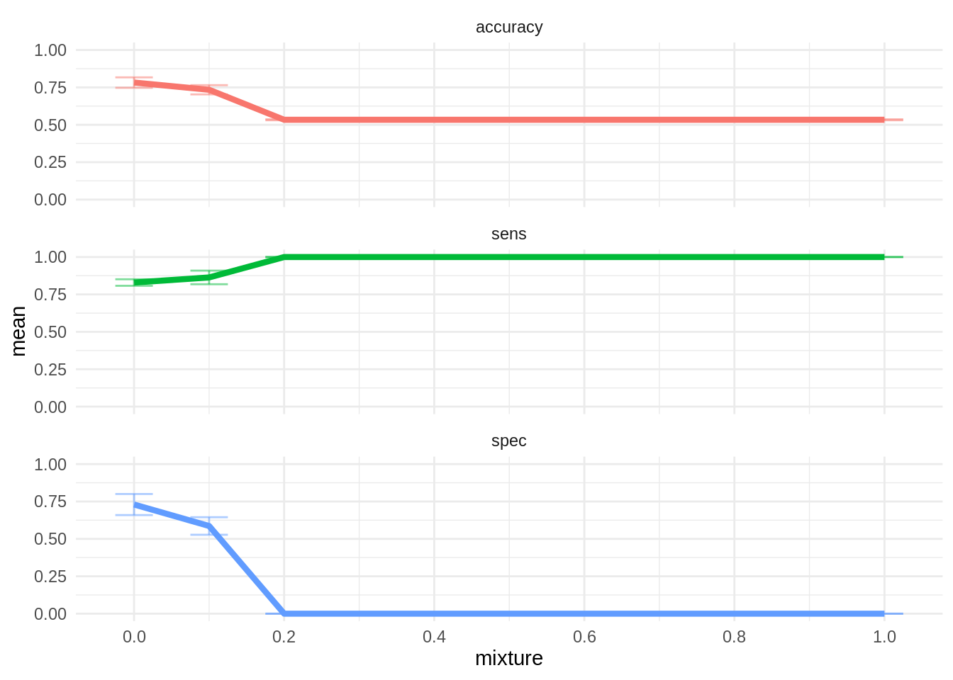
The best model is ridge regression with mixture = 0. The other values of mixture classify all observations as positive, so they are not informative. The fit of this model is better than logistic regression, so we will adopt it as final model.
Training the best model
Let’s train the selected ridge model on the whole train set:
ridge <- logistic_reg(penalty = 1, mixture = 0) %>%
  set_engine("glmnet")

best_model <- workflow() %>%
  add_recipe(recipe) %>%
  add_model(ridge) %>%
  fit(training(split))
Performance on the train set:
best_model %>%
  predict(training(split)) %>%
  bind_cols(training(split)) %>%
  sonar_metrics(truth = Class, estimate = .pred_class)
## # A tibble: 3 × 3
## .metric .estimator .estimate
## <chr> <chr> <dbl>
## 1 accuracy binary 0.824
## 2 sens binary 0.852
## 3 spec binary 0.792Performance on the test set:
best_model %>%
  predict(testing(split)) %>%
  bind_cols(testing(split)) %>%
  sonar_metrics(truth = Class, estimate = .pred_class)
## # A tibble: 3 × 3
## .metric .estimator .estimate
## <chr> <chr> <dbl>
## 1 accuracy binary 0.791
## 2 sens binary 0.826
## 3 spec binary 0.75The metrics on the test set are not much worse than in the train set, so we can assert that the model does not overfit to the train test.
References
- Jun, Kang (2021), tidymodels and glmnet. https://www.jkangpathology.com/post/tidymodel-and-glmnet/
- Kuhn, M.; Vaughan, D. Technical aspects of the glmnet model. https://parsnip.tidymodels.org/reference/glmnet-details.html
- R documentation. Sonar: Sonar, Mines vs. Rocks. https://rdrr.io/cran/mlbench/man/Sonar.html
- Silge, Julia (2021). Add error for ridge regression with glmnet #431. https://github.com/tidymodels/parsnip/issues/431
- Silge, Julia (2020). LASSO regression using tidymodels and #TidyTuesday data for The Office. https://juliasilge.com/blog/lasso-the-office/
Session info
## R version 4.2.0 (2022-04-22)
## Platform: x86_64-pc-linux-gnu (64-bit)
## Running under: Linux Mint 19.2
##
## Matrix products: default
## BLAS:   /usr/lib/x86_64-linux-gnu/openblas/libblas.so.3
## LAPACK: /usr/lib/x86_64-linux-gnu/libopenblasp-r0.2.20.so
##
## locale:
##  [1] LC_CTYPE=es_ES.UTF-8       LC_NUMERIC=C
##  [3] LC_TIME=es_ES.UTF-8        LC_COLLATE=es_ES.UTF-8
##  [5] LC_MONETARY=es_ES.UTF-8    LC_MESSAGES=es_ES.UTF-8
##  [7] LC_PAPER=es_ES.UTF-8       LC_NAME=C
##  [9] LC_ADDRESS=C               LC_TELEPHONE=C
## [11] LC_MEASUREMENT=es_ES.UTF-8 LC_IDENTIFICATION=C
##
## attached base packages:
## [1] stats     graphics  grDevices utils     datasets  methods   base
##
## other attached packages:
##  [1] glmnet_4.1-4       Matrix_1.4-1       mlbench_2.1-3      yardstick_0.0.9
##  [5] workflowsets_0.2.1 workflows_0.2.6    tune_0.2.0         tidyr_1.2.0
##  [9] tibble_3.1.6       rsample_0.1.1      recipes_0.2.0      purrr_0.3.4
## [13] parsnip_0.2.1      modeldata_0.1.1    infer_1.0.0        ggplot2_3.3.5
## [17] dplyr_1.0.9        dials_0.1.1        scales_1.2.0       broom_0.8.0
## [21] tidymodels_0.2.0
##
## loaded via a namespace (and not attached):
##  [1] lubridate_1.8.0    DiceDesign_1.9     tools_4.2.0        backports_1.4.1
##  [5] bslib_0.3.1        utf8_1.2.2         R6_2.5.1           rpart_4.1.16
##  [9] DBI_1.1.2          colorspace_2.0-3   nnet_7.3-17        withr_2.5.0
## [13] tidyselect_1.1.2   compiler_4.2.0     cli_3.3.0          labeling_0.4.2
## [17] bookdown_0.26      sass_0.4.1         stringr_1.4.0      digest_0.6.29
## [21] rmarkdown_2.14     pkgconfig_2.0.3    htmltools_0.5.2    parallelly_1.31.1
## [25] lhs_1.1.5          highr_0.9          fastmap_1.1.0      rlang_1.0.2
## [29] rstudioapi_0.13    farver_2.1.0       shape_1.4.6        jquerylib_0.1.4
## [33] generics_0.1.2     jsonlite_1.8.0     magrittr_2.0.3     Rcpp_1.0.8.3
## [37] munsell_0.5.0      fansi_1.0.3        GPfit_1.0-8        lifecycle_1.0.1
## [41] furrr_0.3.0        stringi_1.7.6      pROC_1.18.0        yaml_2.3.5
## [45] MASS_7.3-57        plyr_1.8.7         grid_4.2.0         parallel_4.2.0
## [49] listenv_0.8.0      crayon_1.5.1       lattice_0.20-45    splines_4.2.0
## [53] knitr_1.39         pillar_1.7.0       future.apply_1.9.0 codetools_0.2-18
## [57] glue_1.6.2         evaluate_0.15      blogdown_1.9       vctrs_0.4.1
## [61] foreach_1.5.2      gtable_0.3.0       future_1.25.0      assertthat_0.2.1
## [65] xfun_0.30          gower_1.0.0        prodlim_2019.11.13 class_7.3-20
## [69] survival_3.2-13    timeDate_3043.102  iterators_1.0.14   hardhat_0.2.0
## [73] lava_1.6.10        globals_0.14.0     ellipsis_0.3.2     ipred_0.9-12