Hypothesis testing is a statistical inference technique to acquire information about a population parameter from observations of a sample, a subet of the population. Let’s suppose that we are testing a new drug to lower blood pressure. We will do that giving the drug to a set of patients on a test group, and a placebo to a test of patients on a control group. We examine the effectiveness of the drug evaluating if it is reasonable to reject the null hypothesis that the mean value of blood pressure in the test group and control group are equal.
There are two types of error in hypothesis testing:
- We commit a Type I error when we reject the null hypothesis when it is true. This means that we are detecting an effect that is not present.
- We commit a Type II error when we do not reject the null hypothesis when it is false. This means that we are not detecting an effect when it is present.
We can control the type I error obtaining a p-value, the probability of observing the obtained value or one more extreme if the hull hypothesis is true.
We reject the null hypothesis if the absolute value of the p-value is smaller than a significance level \(\alpha\). Although the significance level should be fixed by the investigator, the common practice in social sciences is to fix it at \(\alpha = 0.05\). More generally:
- if the absolute value of the p-value is lower than significance level \(\alpha\) we can reject the null hypothesis,
- if the absolute value of the p-value is higher than significance level \(\alpha\), we don’t know if the null hypothesis is true or false.
Family of hypotheses
When doing a statistical analysis, it is frequent that we test a group of \(m\) hypotheses, rather just one. Examples of this are multivariate regression, or a set of experiments with control and experimental groups. A family of hypotheses is a set of hypotheses that are tested together in a statistical analysis.
As we increase the number of hypotheses \(m\), the probability of making at least one Type I er ror increases. Let’s suppose that \(m_0 < m\) null hypotheses are true (this value \(m_0\) is not known by the investigator). The familywise error rate (FWER) is the probability of making at least one Type I error.
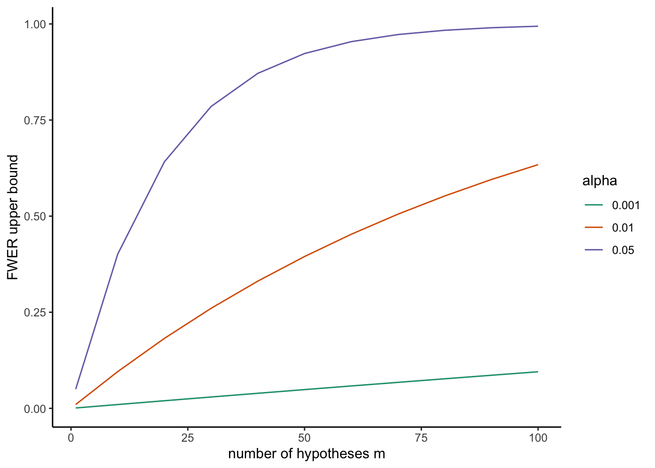
For a significance level \(\alpha\), an upper bound of FWER can be obtained if we set \(m_0 = m\):
\[ 1 - \left(1-\alpha\right)^m \]
Let’s wrap this expression into a function:
mult_test <- \(alpha, m){
  m_alpha <- 1 - (1-alpha)^m
  return(m_alpha)
}
If we have to perform many tests, this upper bound of FWER can escalate quickly:
mult_test(alpha = 0.05, m = 10)## [1] 0.4012631In this plot, I am presenting values of the upper bound of FWER for different values of \(m\) and \(\alpha\).
Bonferroni and Šidák corrections
When we perform tests for a family of hypotheses, we need to reduce the significance level \(\alpha\) of each hypotheses to control the familywise error rate.
The most common method to control FWER is the Bonferroni correction. Although named after Carlo Emilio Bonferroni for being grounded on the Bonferroni inequalities, the correction is attributed to Olive Jean Dunn. This correction consists simply of lowering the significance level to:
\[\alpha_{BON} = \alpha/m\]
So, if we have \(m=20\) tests of hypotheses and \(\alpha=0.05\), we need to reset the significance level of each test to \(\alpha/m = 0.05/20 = 0.0025\).
This correction can be considered too restrictive for two reasons:
- Assumes that all null hypotheses are true,
- and leads to a FWER smaller to the original \(\alpha\). For \(m=20\) we have:
mult_test(alpha = 0.05/20, m = 20)## [1] 0.04883012To account for this later effect, we can use the Šidák correction, developed by Zbyněk Šidák. The significance level for each test is defined as:
\[ \alpha_{SID} = 1 - \left( 1 - \alpha \right)^{\frac{1}{m}} \]
For \(\alpha = 0.05\) and \(m=20\) we have a value of Šidák correction:
alpha_sidak <- 1 - (1-0.05)^{1/20}
alpha_sidak
## [1] 0.002561379This value is slightly larger than the obtained with the Bonferroni correction, so we are gaining some statistical power.
mult_test(alpha = alpha_sidak, m = 20)## [1] 0.05The Holm-Bonferroni method
Developed by Sture Holm, this method aims to control FWER in a less stringent way than the Bonferroni and Šidák corrections, thus gaining statistical power for the family of test of hypotheses. It is an interative method, when we adjust the significance level at each step:
- Sorting the p-values in non-decreasing order (from smallest to largest) \(P_1, P_2, \dots, P_m\).
- For \(k=1, \dots, m\) check if \(P_k < \alpha/\left(m+1-k\right)\), reject the hypothesis if it is true and stop the procedure when it is false.
Example of application
Let’s suppose that we have performed a family of test of hypotheses and we have obtained the following p-values:
pvalues <- c(0.01, 0.04, 0.03, 0.005)If we set \(\alpha = 0.05\), we will reject all four, and therefore we will assume that all effects are significant. But as we are doing the four tests together, the probability of making at least one Type I error is equal to:
mult_test(alpha = 0.05, m = 4)## [1] 0.1854938In the following table, we will see the results of applying the three methods described here to limit the familywise error rate.
| test | p-values | Bonf | Šidák | Holm |
|---|---|---|---|---|
| P4 | 0.005 | 0.0125 | 0.0127415 | 0.0125000 |
| P1 | 0.010 | 0.0125 | 0.0127415 | 0.0166667 |
| P3 | 0.030 | 0.0125 | 0.0127415 | 0.0250000 |
| P2 | 0.040 | 0.0125 | 0.0127415 | 0.0500000 |
From the results of the table, we can conclude that:
- We will accept all null hypothesis if we use the Bonferroni and Šidák methods.
- We will reject hypothesis 4 and 1, but not 3 and 2 if we use the Holm-Bonferroni method. Note that we stop the method with \(P_3\), so we do not asses \(P_2\).
In this example we can appreciate how the Bonferroni and Šidák methods are conservative when it comes to reject null hypotheses when a family of these is examined together. The Holm-Bonferroni method is less conservative, and allows to take into account the effect of multiple testing loosing a smaller amount statistical power.
References
- Amat Rodrigo, J. (2016). Comparaciones múltiples: corrección de p-value y FDR https://rpubs.com/Joaquin_AR/236898.
- Dunn, Olive Jean (1961). Multiple Comparisons Among Means. Journal of the American Statistical Association. 56 (293): 52–64.
- Glen, Stephanie. Holm-Bonferroni Method: Step by Step, StatisticsHowTo.com: Elementary Statistics for the rest of us! https://www.statisticshowto.com/holm-bonferroni-method/. Retrieved at 2021-09-23.
- Holm, S. (1979). A simple sequentially rejective multiple test procedure. Scandinavian Journal of Statistics. 6 (2): 65–70.
- Šidák, Z. K. (1967). Rectangular Confidence Regions for the Means of Multivariate Normal Distributions. Journal of the American Statistical Association. 62 (318): 626–633. doi:10.1080/01621459.1967.10482935.
Built with R 4.1.0, dplyr 1.0.7, ggplot2 3.3.4, kableExtra 1.3.4 and RColorBrewer 1.1-2