In a previous post I have introduced the graph coloring problem and used a linear programming formulation to apply this problem to color a map of districts of Barcelona. In this post, I will try to color the map of neighbourhoods (barris) of Barcelona solving a graph coloring problem. In addition to the tidyverse for data handling and BAdatasetsSpatial to get the map, I will be using sf for spatial data handling and tidygraph and ggraph to work with graphs.
library(tidyverse)
library(BAdatasetsSpatial)
library(sf)

library(tidygraph)
library(ggraph)
Firstly, I will get the neighbourhoods, stored in the BCNNeigh sf object.
data("BCNNeigh")

BCNNeigh <- BCNNeigh |>
  arrange(c_barri)

int <- st_touches(BCNNeigh)

edges_bcn <- map_dfr(1:length(int), ~ tibble(i = ., j = int[[.]])) |>
  filter(i < j) # 195 edges

edges_bcn <- edges_bcn |>
  mutate(id = 1:n())
The map has up to 73 zones, stacked in complicated ways specially at the north.
BCNNeigh |>
  ggplot() +
  geom_sf(fill = "white") +
  geom_text(aes(coord_x, coord_y, label = c_barri), size = 3) +
  theme_void() +
  theme(legend.position = "none")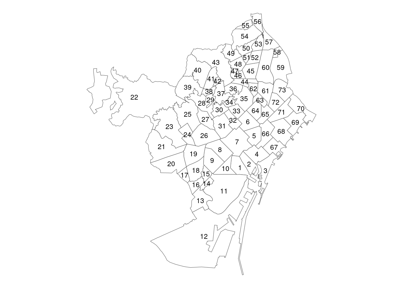
To solve the graph coloring problem, we need to define a graph with a node for each spatial region connected by edges if they touch each other. If we represent the graph, we observe that it is non-planar, as some edges cross each other. This is because some regions are connected by a single point, and it is correct to use the same color to label them. The edges representing one-point connections are plotted in red.
bcn_neigh_graph <- tbl_graph(edges = edges_bcn, directed = TRUE)

bcn_neigh_graph <- bcn_neigh_graph |>
  activate(nodes) |>
  mutate(label = 1:n())

bcn_neigh_graph <- bcn_neigh_graph |>
  activate(edges) |>
  mutate(label = 1:n())

non_planar_edges <- c(140, 144, 151, 147, 153, 158, 54, 112, 116)

bcn_neigh_graph <- bcn_neigh_graph |>
  activate(edges) |>
  mutate(planar = ifelse(label %in% non_planar_edges, "no", "yes"))

m_layout <- matrix(c(BCNNeigh$coord_x, BCNNeigh$coord_y), ncol = 2)

ggraph(bcn_neigh_graph, layout = m_layout) +
  geom_edge_link(aes(color = planar),
                 start_cap = circle(2, "mm"),
                 end_cap = circle(2, "mm")) +
  geom_node_text(aes(label = label), size = 3) +
  scale_edge_color_manual(values = c("#FF0000", "#808080")) +
  theme_graph() +
  theme(legend.position = "none")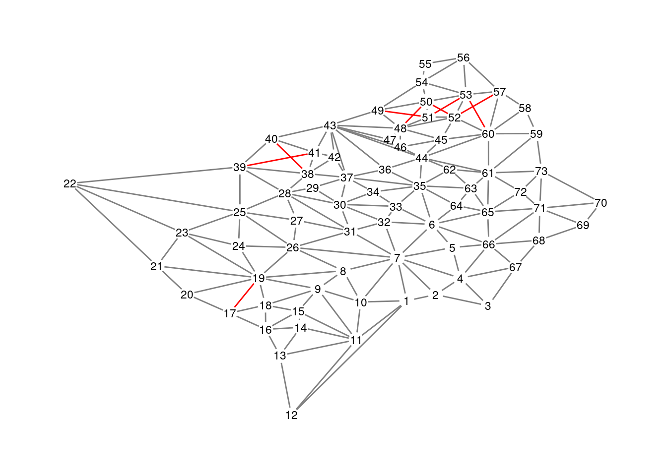
We remove the edges in red to get a planar graph, edges_non_planar.
edges_bcn_planar <- edges_bcn |>
  filter(!id %in% non_planar_edges)
A Greedy Algorithm for the Graph Coloring Problem
The instance is too large and intricate to solve it using linear programming, so we can try a constructive heuristic. It is defined as follows:
- Label the first node with the first color.
- For the remaining nodes:
- Consider each node, and color it with the color of lowest number not used in adjacent nodes colored previously. If all colors used so far appear in the adjacent, yet colored nodes, assing the node a new color.
This heuristic is implemented in the gc_heuristic() function.
gc_heuristic <- function(edges_col){

  nodes <- sort(unique(c(edges_col$i, edges_col$j)))
  n_nodes <- length(nodes)
  color <- c(1, rep(0, n_nodes - 1))

  for(i in 2:(n_nodes)){

    node_to_color <- nodes[i]

    # nodes adjacent to node_to_color
    adj_table <- edges_col |>
      filter(i == node_to_color | j == node_to_color)
    adj_nodes <- unique(c(adj_table$i, adj_table$j))

    # nodes adjacent to node_to_color colored previously
    adj_nodes <- adj_nodes[which(adj_nodes %in% nodes[1:(i-1)])]

    #colores usados en los vertices adyacentes coloreados previamente
    prev_colors <- color[which(nodes %in% adj_nodes)] |> unique()
    new_color <- which(!1:n_nodes %in% prev_colors) |> min()
    color[i] <- new_color
  }

  solution <- tibble(node = nodes,  color = color)
  return(solution)
}
Let’s obtain the solution of our problem with this heuristic:
sol <- gc_heuristic(edges_bcn_planar)We observe that we have needed five colors to solve the problem:
unique(sol$color)## [1] 1 2 3 4 5A Tabu Search Algorithm for the Graph Coloring Problem
With the constructive heuristic we have obtained a way to color the map using five colors. But we know that the chromatic number (minimum number of colors) of a planary graph is four. To improve the five color solution, I have defined a tabu search heuristic for the graph coloring problem.
In this heuristic, we fix the number of colors n_c and we aim to minimize the number of edges with nodes with the same color. This value is obtained with the edges_invalid() function. We get the coloring with n_c colors when this objective function is equal to zero.
The neighborhood of a solution has all nodes with the same color except one node. So in each iteration we test the objective function for each node and each color different from the one in the current solution. The tabu search is implemented in the tabu_gc() function.
edges_invalid <- function(edges_col, solution){

  t1 <- left_join(edges_col, solution, by = c("i" = "node"))
  t1 <- left_join(t1, solution, by = c("j" = "node"))
  ie <- sum(t1$color.x == t1$color.y)
  return(ie)
}

tabu_gc <- function(edges_col, n_c, iter, tabu_size, verbose = FALSE){

  # nodes of instance and number of nodes
  nodes <- sort(unique(c(edges_col$i, edges_col$j)))
  n_nodes <- length(nodes)

  # starting solution
  inisol <- gc_heuristic(edges_col)

  inisol <- inisol |>
    mutate(color = ifelse(color > n_c, n_c, color))

  #list of moves
  moves <- map_dfr(1:n_c, ~ bind_cols(tibble(node = nodes, color = .)))
  moves <- moves |>
    mutate(id = 1:n()) |>
    relocate(id)

  ##setting starting value of sol, fit, bestsol and bestfit
  sol <- inisol
  fit <- edges_invalid(edges_col, sol)
  bestsol <- inisol
  bestfit <- fit
  evalfit <- fit
  evalbest <- bestfit

  #initializing tabu list
  tabu_list <- rep(0, tabu_size)

  ##setting counters
  count <- 1
  count_tlist <- 0

  while(count <= iter & bestfit > 0){

    # nodes to explore not belonging to solution
    exploring_moves <- anti_join(moves, sol, by = c("node", "color"))

    # computing fitness for each mov
    exploring_moves <- exploring_moves |>
      mutate(fit = pmap_int(exploring_moves, ~ {
        test_sol <- sol |>
          filter(node != ..2)
        test_sol <- bind_rows(test_sol, tibble(node = ..2, color = ..3))
        ie <- edges_invalid(edges_col, test_sol)
        return(ie)
      }))

    exploring_moves <- exploring_moves |>
      arrange(fit)

    best_not_tabu <- exploring_moves |>
      filter(!id %in% tabu_list) |>
      slice(1)

    best_tabu <- exploring_moves |>
      filter(id %in% tabu_list) |>
      slice(1)

    if(nrow(best_tabu) == 0)
      best_tabu <- data.frame(id = 0, node = 0, color = 0, fit = Inf)

    if(best_tabu$fit < bestfit){
      sol <- sol |>
        filter(node != best_tabu$node)
      sol <- bind_rows(sol, best_tabu |> select(-c(fit, id)))
      fit <- best_tabu$fit
      asp <- TRUE
    }else{
      sol <- sol |>
        filter(node != best_not_tabu$node)
      sol <- bind_rows(sol, best_not_tabu |> select(-c(fit, id)))
      fit <- best_not_tabu$fit
      asp <- FALSE
    }

    if(fit < bestfit){
      bestsol <- sol
      bestfit <- fit
    }

    ##update tabu list
    if(!asp){
      tabu_list[count_tlist %% tabu_size + 1] <- best_not_tabu$id
      count_tlist <- count_tlist + 1
    }

    if(verbose)
      cat("iteration: ", count, " fit: ", bestfit, "\n")

    evalfit <- c(evalfit, fit)
    evalbest <- c(evalbest, bestfit)
    count <- count + 1
  }

  fit_track <- data.frame(step = 1:length(evalfit), fit = evalfit, best = evalbest)

  return(list(sol = bestsol, fit = bestfit, fit_track = fit_track))
  ## return solution if feasible solution is found
}
Let’s find the solution with the tabu search heuristic:
tabu_sol <- tabu_gc(edges_col = edges_bcn_planar, n_c = 4, iter = 200, tabu_size = 100)This new solution has four colors:
unique(tabu_sol$sol$color)## [1] 1 4 2 3The following plot presents the evolution of the algorithm. It has explored solutions with up to five edges with the same color until finding the optimum.
tabu_sol$fit_track |>
  pivot_longer(-step) |>
  ggplot(aes(step, value, color = name)) +
  geom_line() +
  theme_minimal(base_size = 12) +
  scale_color_manual(name = "colors", values = c("#CC0000", "#0080FF"))  +
  theme(legend.position = "bottom") +
  labs(title = "Tabu Search Algorithm", x = NULL, y = NULL)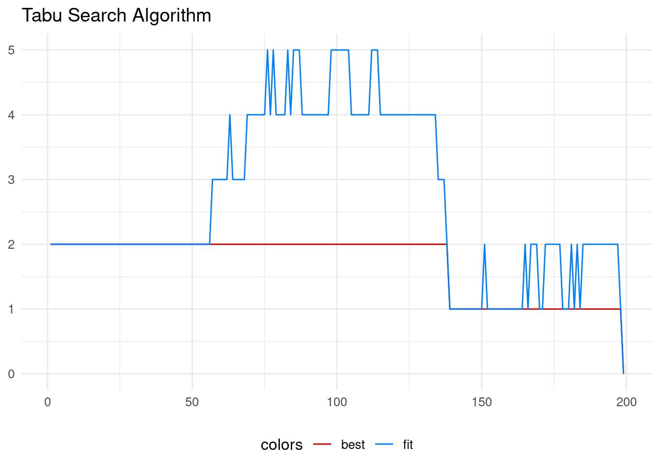
Now it’s time to plot the map. First, we attach the labelling to the BCNNeigh table:
BCNNeigh <- left_join(BCNNeigh,
                      tabu_sol$sol,
                      by = c("c_barri" = "node"))
And finally we obtained the colored map.
BCNNeigh |>
  ggplot() +
  geom_sf(aes(fill = factor(color))) +
  theme_void() +
  theme(legend.position = "none") +
  scale_fill_brewer(palette = "Reds")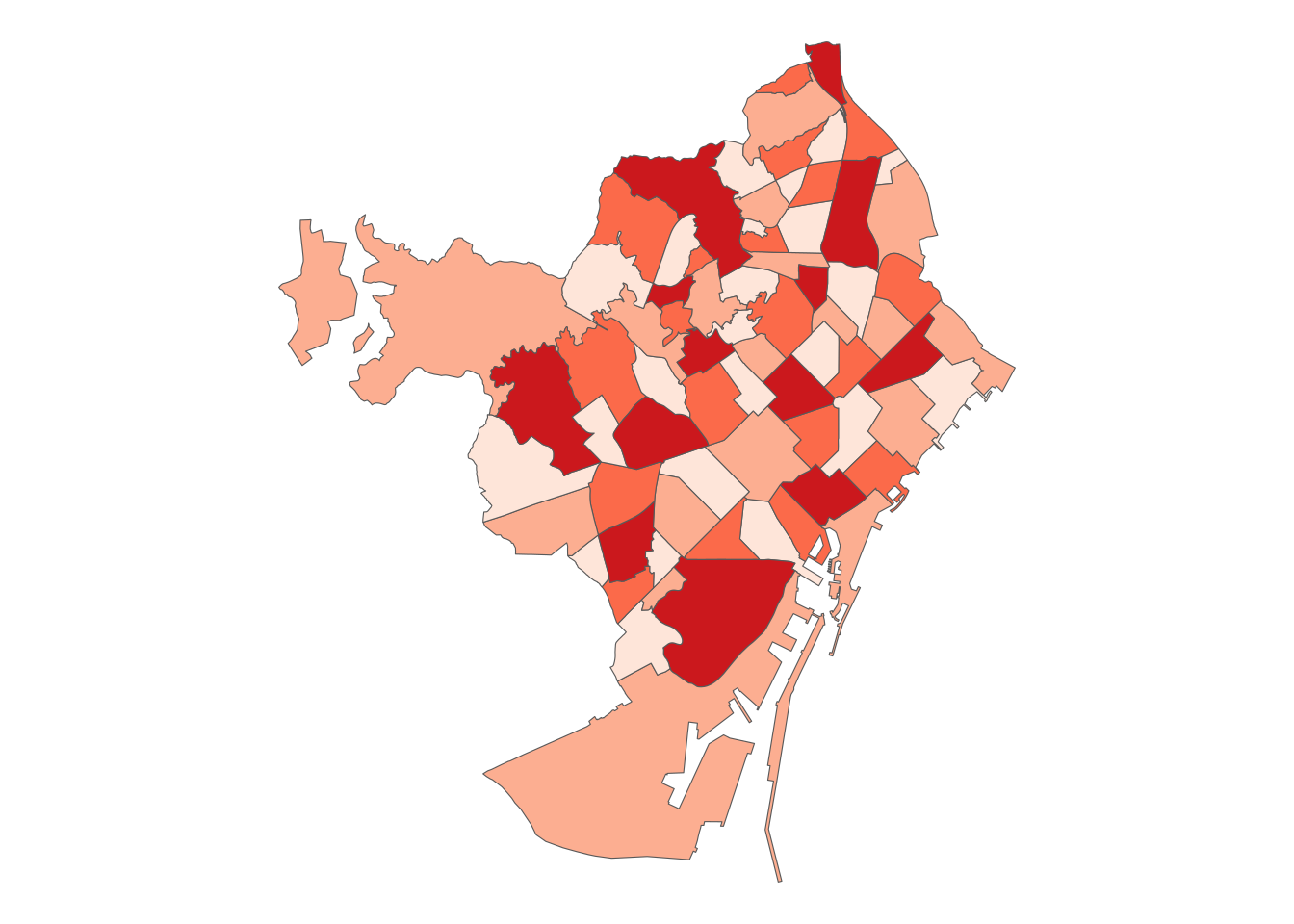
Map Coloring with the Graph Coloring Problem
In two posts, I have presented how to color a map using the graph coloring problem. We know that the chromatic number of a planar graph is no larger than four. To be planar, the edges of the graph must not cross. In this particular case, I have to remove some edges obtained with spatial analysis to make the graph planar and finding a coloring with four numbers.
In the previous post, I used linear programming to solve a small instance with 10 nodes and 19 connections. This instance is much larger, of 73 nodes with 186 observations. The linear programming formulation does not scale up to a problem of this size, so I needed to define a constructive heuristic to obtain a starting solution, and later refine it with a local search algorithm based on the tabu search metaheurisic.
Reference
- Node coloring with linear programming https://jmsallan.netlify.app/blog/node-coloring-with-linear-programming/
Session Info
## R version 4.4.1 (2024-06-14)
## Platform: x86_64-pc-linux-gnu
## Running under: Linux Mint 21.1
##
## Matrix products: default
## BLAS:   /usr/lib/x86_64-linux-gnu/blas/libblas.so.3.10.0
## LAPACK: /usr/lib/x86_64-linux-gnu/lapack/liblapack.so.3.10.0
##
## locale:
##  [1] LC_CTYPE=es_ES.UTF-8       LC_NUMERIC=C
##  [3] LC_TIME=es_ES.UTF-8        LC_COLLATE=es_ES.UTF-8
##  [5] LC_MONETARY=es_ES.UTF-8    LC_MESSAGES=es_ES.UTF-8
##  [7] LC_PAPER=es_ES.UTF-8       LC_NAME=C
##  [9] LC_ADDRESS=C               LC_TELEPHONE=C
## [11] LC_MEASUREMENT=es_ES.UTF-8 LC_IDENTIFICATION=C
##
## time zone: Europe/Madrid
## tzcode source: system (glibc)
##
## attached base packages:
## [1] stats     graphics  grDevices utils     datasets  methods   base
##
## other attached packages:
##  [1] ggraph_2.2.1            tidygraph_1.3.1         sf_1.0-16
##  [4] BAdatasetsSpatial_0.1.0 lubridate_1.9.3         forcats_1.0.0
##  [7] stringr_1.5.1           dplyr_1.1.4             purrr_1.0.2
## [10] readr_2.1.5             tidyr_1.3.1             tibble_3.2.1
## [13] ggplot2_3.5.1           tidyverse_2.0.0
##
## loaded via a namespace (and not attached):
##  [1] gtable_0.3.5       xfun_0.43          bslib_0.7.0        ggrepel_0.9.5
##  [5] tzdb_0.4.0         vctrs_0.6.5        tools_4.4.1        generics_0.1.3
##  [9] proxy_0.4-27       fansi_1.0.6        highr_0.10         pkgconfig_2.0.3
## [13] KernSmooth_2.23-24 RColorBrewer_1.1-3 lifecycle_1.0.4    compiler_4.4.1
## [17] farver_2.1.1       munsell_0.5.1      ggforce_0.4.2      graphlayouts_1.1.1
## [21] htmltools_0.5.8.1  class_7.3-22       sass_0.4.9         yaml_2.3.8
## [25] pillar_1.9.0       jquerylib_0.1.4    MASS_7.3-60        classInt_0.4-10
## [29] cachem_1.0.8       wk_0.9.1           viridis_0.6.5      tidyselect_1.2.1
## [33] digest_0.6.35      stringi_1.8.3      bookdown_0.39      labeling_0.4.3
## [37] polyclip_1.10-6    fastmap_1.1.1      grid_4.4.1         colorspace_2.1-0
## [41] cli_3.6.2          magrittr_2.0.3     utf8_1.2.4         e1071_1.7-14
## [45] withr_3.0.0        scales_1.3.0       timechange_0.3.0   rmarkdown_2.26
## [49] igraph_2.0.3       gridExtra_2.3      blogdown_1.19      hms_1.1.3
## [53] memoise_2.0.1      evaluate_0.23      knitr_1.46         viridisLite_0.4.2
## [57] s2_1.1.6           rlang_1.1.3        Rcpp_1.0.12        glue_1.7.0
## [61] DBI_1.2.2          tweenr_2.0.3       rstudioapi_0.16.0  jsonlite_1.8.8
## [65] R6_2.5.1           units_0.8-5