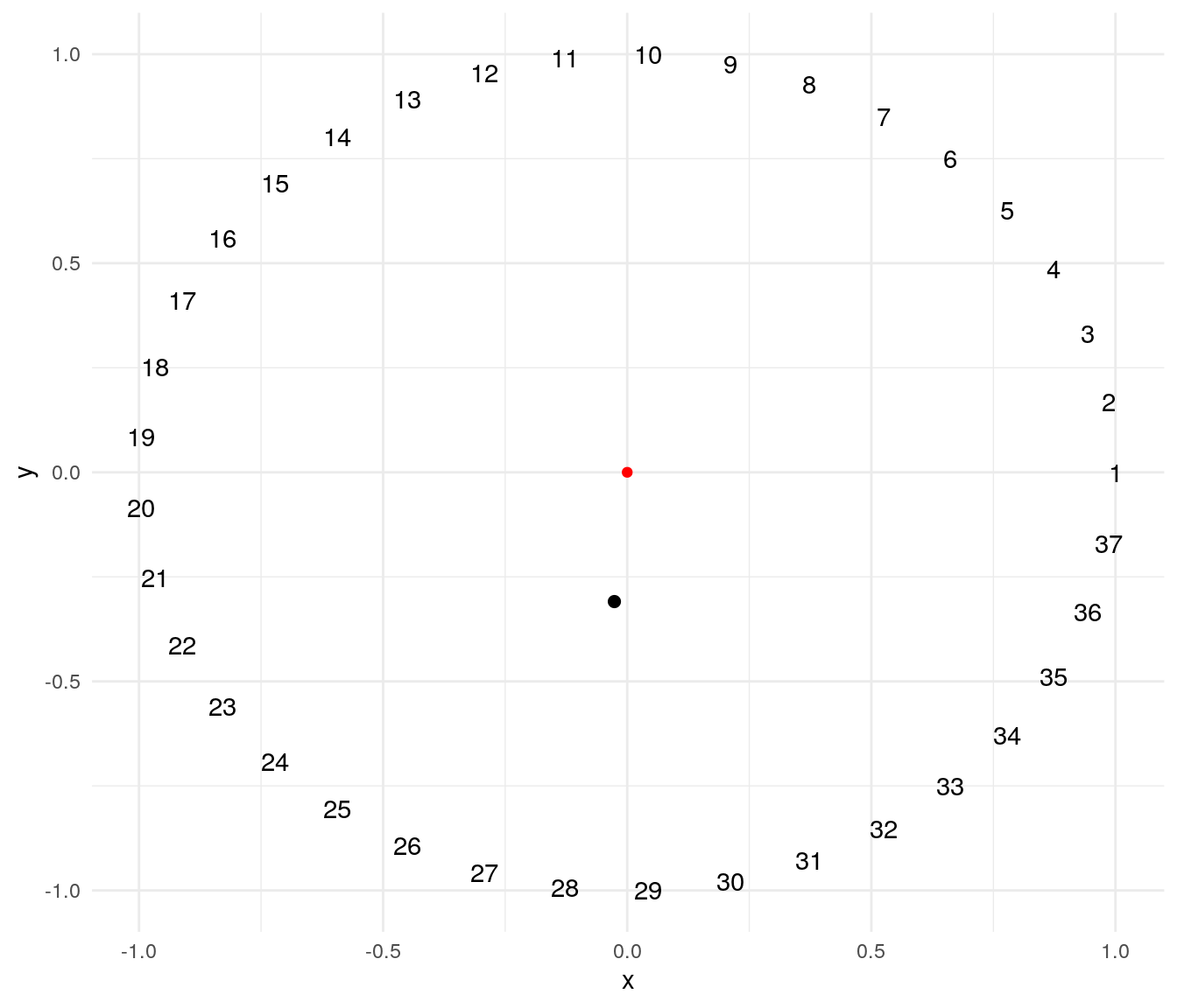
To illustrate this technique I will use a problem suggested by professor Éric Taillard. The problem consists of ordering \(n\) masses of weights \(1, 2, \dots, n\) evenly on a circumference so that the distance of the center of mass to the center of the circle is minimized. The plot below presents a possible solution for a problem of \(n=37\). The red point of is the center of the circle, and the black point is the center of mass of the solution.
A solution of this problem can be encoded as a cyclic permutation, where the first element is fixed and the remaining \(n-1\) elements can take any order. The mass_center function returns the distance to the origin of the center of mass of a possible solution:
mass_center <- function(v){
  n <- length(v)

  angles <- 0:(n-1) * 2 * pi / n
  x <- v*cos(angles)
  y <- v*sin(angles)
  dcm <- c(sum(x), sum(y))/sum(v)
  dcm <- sqrt(sum(dcm^2))

  return(dcm)
}
The distance of the mass center to the center for the solution of the plot above is:
mass_center(1:37)## [1] 0.310306A steepest descent algorithm
The implementation of a local search algorithm requires defining the neighborhood of a solution, the set of solutions that can be explored from a specific solution. We can define a neighborhood with the swap operator:
swap <- function(v, i , j){

  aux <- v[i]
  v[i] <- v[j]
  v[j] <- aux
  return(v)
}
As the swap operator is permutative and \(i \neq j\), from one solution we can explore \(\left(n-1 \right)\left(n-2 \right)/2\) different solutions.
A steepest descent algorithm explores all the solutions of a neighborhood of the current solution \(x\) and picks as next solution to explore the best solution of the neighbourhood \(x'\).
The function sd_circle implements the steepest descent algorithm for the center of mass problem. The solution to explore at each step is sol, the best solution of the neighborhood is testsol and the best solution found is bestsol. The algorithm stops when the solution does not improve after iter steps.
sd_circle <- function(inisol, iter = 100, eval = TRUE){

  #tracking evaluation
  if(eval){
    evalfit <- numeric()
    evalbest <- numeric()
  }

  #initialization
  n <- length(inisol)
  sol <- inisol
  bestsol <- inisol
  bestfit <- mass_center(sol)
  T <- 1

  while(T <= iter){

    #find the best move
    fit <- Inf
    bestmove <- c(0,0)

    #examining all swap moves on a cyclic permutation
    for(i in 2:(n-1))
        for(j in (i+1):n){

          testsol <- swap(sol, i, j)
          testfit <- mass_center(testsol)

          if(testfit <= fit){
            fit <- testfit
            bestmove <- c(i, j)
          }
        }

    #the new solution to explore is the best found
    sol <- swap(sol, bestmove[1], bestmove[2])

    #update best solution
    if(fit < bestfit){
      bestsol <- sol
      bestfit <- fit
    }

    T <- T + 1

    #track evaluation

    if(eval){
      evalfit <- c(evalfit, fit)
      evalbest  <- c(evalbest, bestfit)
    }
  }

  #return solution
  if(eval)
    return(list(sol=bestsol, fit=bestfit, evalfit=evalfit, evalbest=evalbest))
  else
    return(list(sol=bestsol, fit=bestfit))

}
Let’s apply the algorithm to an instance of size 37.
sd_test <- sd_circle(inisol = 1:37)The solution obtained is quite good:
sd_test$fit## [1] 3.654601e-05If we examine the evolution of this algorithm we see that it converges to a local optimum, a solution whose fit is better than any solution of its neighborhood. In fact, the steepest descent algorithm can stop when the fit of all the elements of the neighborhood do not improve the one of \(x\). As the scale of the solution obtained changes in the first iterations, I am presenting the logarithm of the objective function.
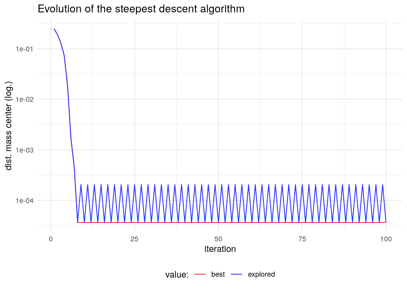
In the first iterations, the algorithm reaches a local optimum. It is a solution that cannot be improved with elements of its neighbourhood. From then on, the algorithm is cycling between the local optimum and the previous solution.
Making moves tabu
The strategy followed by tabu search is to avoid cycling by prohibiting (making tabu) the moves that undo the moves made previous iterations. These moves are stored in a tabu list. Tabu search, unlike simulated annealing or steepest descent, is an algorithm with memory of its evolution.
The way we store tabu moves depends on the way we define the neighbourhood. In a swap move, we observe that a swap \(\left(i,j\right)\) is undone by the same swap \(\left(i,j\right)\). Let’s see what happens when we swap a vector a into b, and perform the same swap into b to get c:
a <- 1:10
b <- swap(a, 4, 8)
c <- swap(b, 4, 8)
cat("a = ", a, "\n")
## a = 1 2 3 4 5 6 7 8 9 10cat("b = ", b, "\n")## b = 1 2 3 8 5 6 7 4 9 10cat("c = ", c, "\n")## c = 1 2 3 4 5 6 7 8 9 10We need to store the moves \(\left(i,j\right)\) in a tabu list, and exclude from searching these moves to escape local optima.
A refinement of the tabu search is to accept some tabu moves if they meet an aspiration condition. A possible aspiration condition is that the tabu move leads to improve the best solution found so far.
Implementing a tabu search algorithm
The ts_circle function implements a tabu search algorithm for the center of mass problem. The function takes the following arguments:
- a starting
solution inisol. iter, the number of examinations of the entire neighbbourhood of a solution without improvement of the best solution found.- the size of the tabu list
tabu_size. - a flag
aspindicating whether we adopt the aspiration condition. If true, we cansider moves that are tabu improving the best solution found so far. - an
evalflag to select if we want to tract the evolution of the algorithm.
The tabu list consists of a tabu_list matrix of two columns and tabu_size rows. It is initialized with non-existing moves, and is updated if the aspiration condition is not met. We examine if a move is tabu with the check_tabu funciton.
ts_circle <- function(inisol, iter=50, tabu_size=5, asp=TRUE, eval=TRUE){
#tracking evaluation
if(eval){
evalfit <- numeric()
evalbest <- numeric()
}
#initialization
sol <- inisol
bestsol <- inisol
bestfit <- mass_center(sol)
T <- 1
Ttabu <- 1
flag_tabu <- FALSE
tabu_list <- matrix(numeric(2*tabu_size), tabu_size, 2)
#function that checks if move v is included in a tabu list M
check_tabu <- function(M, v) any(colSums(apply(M, 1, function(x) v == x))==2)
n <- length(sol)
while (T<=iter){
found_best <- FALSE
#find the best move
fit <- Inf
bestmove <- c(0,0)
#examining all swap moves
for(i in 2:(n-1))
for(j in (i+1):n){
testsol <- swap(sol, i, j)
testfit <- mass_center(testsol)
#improvement with non-tabu move
if(testfit <= fit & check_tabu(tabu_list, c(i,j))==FALSE){
fit <- testfit
bestmove <- c(i, j)
flag_tabu <- TRUE
}
#improvement with tabu move, and aspiration condition
if(testfit < bestfit & check_tabu(tabu_list, c(i,j))==TRUE & asp==TRUE){
fit <- testfit
bestmove <- c(i, j)
flag_tabu <- FALSE
}
}
#obtain sol
sol <- swap(sol, bestmove[1], bestmove[2])
#update bestsol
if(fit < bestfit){
bestfit <- fit
bestsol <- sol
found_best <- TRUE
T <- 1
}else{
T <- T + 1
}
#update tabu list
if(flag_tabu){
tabu_list[Ttabu%%tabu_size+1, ] <- bestmove
Ttabu <- Ttabu + 1
}
#track evaluation
if(eval){
evalfit <- c(evalfit, fit)
evalbest <- c(evalbest, bestfit)
}
}
if(eval)
return(list(sol=bestsol, fit=bestfit, evalfit=evalfit, evalbest=evalbest))
else
return(list(sol=bestsol, fit=bestfit))
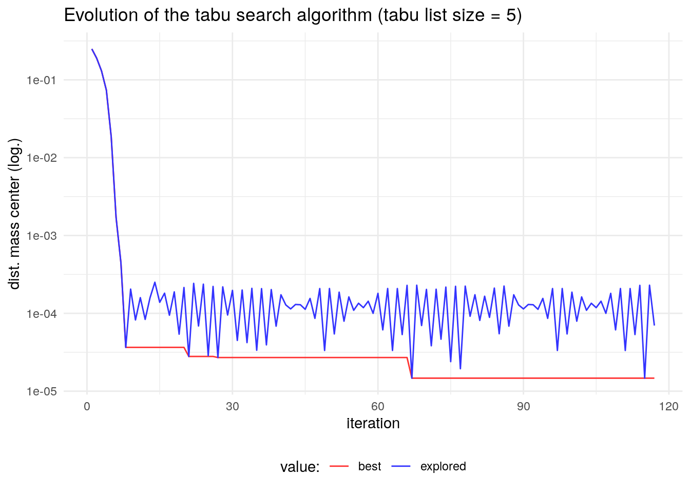
}Let’s apply ts_circle to a problem of size 37. Unlike other metaheuristics like simulated annealing, tabu search is deterministic so we don’t need to set the seed of random numbers.
ts_test <- ts_circle(inisol = 1:37)The value of the objective function is better than the obtained with steepest descent:
ts_test$fit## [1] 1.470133e-05This improvement is achieved by breaking the cyclicity of the evolution of the steepest descent algorithm. Here wee see that the algorithm ends up cycling in the end, but with a larger period.
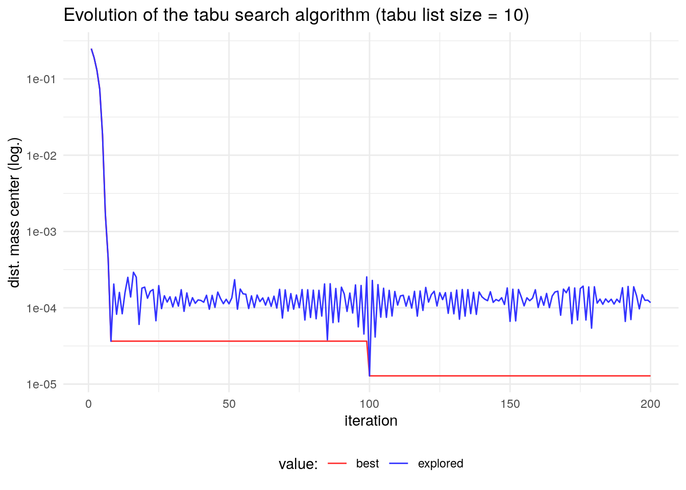
Let’s try to find a better solution with a larger tabu size, and more iterations before stopping. This later condition will make the algorithm take more time to run.
ts_test2 <- ts_circle(inisol = 1:37, iter = 100, tabu_size = 10)We observe an improvement of the obtained solution:
ts_test2$fit## [1] 1.282861e-05The evolution of the algorithm demonstrates that in this case increasing the tabu size leads to a better search of the solution space and therefore a better solution.
References
- Professor Éric Taillard’s website: http://mistic.heig-vd.ch/taillard/
Session info
## R version 4.1.2 (2021-11-01)
## Platform: x86_64-pc-linux-gnu (64-bit)
## Running under: Debian GNU/Linux 10 (buster)
##
## Matrix products: default
## BLAS:   /usr/lib/x86_64-linux-gnu/blas/libblas.so.3.8.0
## LAPACK: /usr/lib/x86_64-linux-gnu/lapack/liblapack.so.3.8.0
##
## locale:
##  [1] LC_CTYPE=es_ES.UTF-8       LC_NUMERIC=C
##  [3] LC_TIME=es_ES.UTF-8        LC_COLLATE=es_ES.UTF-8
##  [5] LC_MONETARY=es_ES.UTF-8    LC_MESSAGES=es_ES.UTF-8
##  [7] LC_PAPER=es_ES.UTF-8       LC_NAME=C
##  [9] LC_ADDRESS=C               LC_TELEPHONE=C
## [11] LC_MEASUREMENT=es_ES.UTF-8 LC_IDENTIFICATION=C
##
## attached base packages:
## [1] stats     graphics  grDevices utils     datasets  methods   base
##
## other attached packages:
## [1] ggplot2_3.3.5 tidyr_1.1.4   dplyr_1.0.7
##
## loaded via a namespace (and not attached):
##  [1] highr_0.9         pillar_1.6.4      bslib_0.2.5.1     compiler_4.1.2
##  [5] jquerylib_0.1.4   tools_4.1.2       digest_0.6.27     jsonlite_1.7.2
##  [9] evaluate_0.14     lifecycle_1.0.0   tibble_3.1.5      gtable_0.3.0
## [13] pkgconfig_2.0.3   rlang_0.4.12      DBI_1.1.1         yaml_2.2.1
## [17] blogdown_1.5      xfun_0.23         withr_2.4.2       stringr_1.4.0
## [21] knitr_1.33        generics_0.1.0    vctrs_0.3.8       sass_0.4.0
## [25] grid_4.1.2        tidyselect_1.1.1  glue_1.4.2        R6_2.5.0
## [29] fansi_0.5.0       rmarkdown_2.9     bookdown_0.24     farver_2.1.0
## [33] purrr_0.3.4       magrittr_2.0.1    scales_1.1.1      ellipsis_0.3.2
## [37] htmltools_0.5.1.1 assertthat_0.2.1  colorspace_2.0-1  labeling_0.4.2
## [41] utf8_1.2.1        stringi_1.7.3     munsell_0.5.0     crayon_1.4.1