A strategy to solve optimization problems is local search. It starts with a solution, that can be built at random or obtained with another heuristic, and tries to improve it iteratively, trying to find solutions with a better fit than the one we are examining belonging to its neighbourhood. Effective local search procedures may explore solutions worse than the one they have found so far, hoping to escape from local optima.
A well-known local search metaheuristic is simulated annealing. Its name comes from annealing in metallurgy, a technique involving heating and controlled cooling of a material to alter its physical properties. The cooling metaphor suggests that the probability of exploring a worse solution decreases with the number of iterations.
To illustrate this technique I will use a problem suggested by professor Éric Taillard. The problem consists of ordering \(n\) masses of weights \(1, 2, \dots, n\) evenly on a circumference so that the distance of the center of mass to the center of the circle is minimized. The plot below presents a possible solution for a problem of \(n=37\). The red point of is the center of the circle, and the black point is the center of mass of the solution.
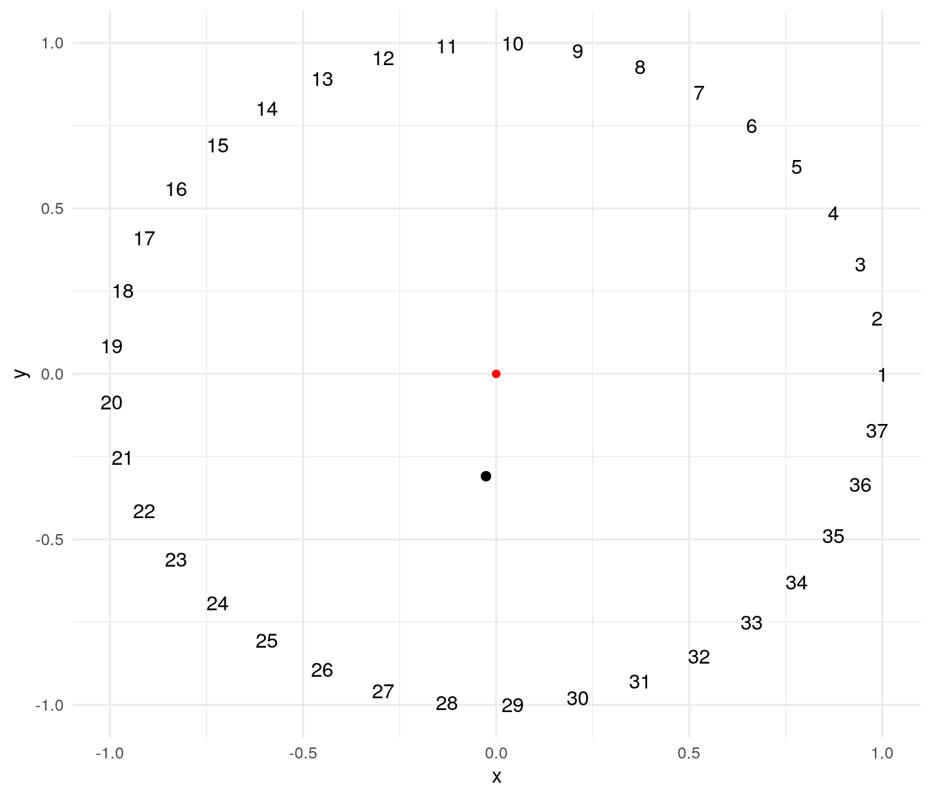
A solution of this problem can be encoded as a cyclic permutation, where the first element is fixed and the remaining \(n-1\) elements can take any order. The mass_center function returns the distance to the origin of the center of mass of a possible solution:
mass_center <- function(v){
  n <- length(v)

  angles <- 0:(n-1) * 2 * pi / n
  x <- v*cos(angles)
  y <- v*sin(angles)
  dcm <- c(sum(x), sum(y))/sum(v)
  dcm <- sqrt(sum(dcm^2))

  return(dcm)
}
The distance of the mass center to the center for the solution of the plot above is:
mass_center(1:37)## [1] 0.310306A simulated annealing heuristic
Let’s use the simmulated annealing metaheuristic to construct a heuristic for this problem. If the fitness function of the problem is \(F\left(x\right)\) we have:
- the solution we are exploring at the moment \(x\) and its fitness function \(f=F\left(x\right)\). These are labelled
solandfitin thesa_circlefunction code. - the best solution we have found so far \(x^{*}\) and its fitness function \(f^{*}=F\left(x^{*}\right)\). They are labeled
bestsolandbestfitin thesa_circlefunction code. - the solution \(x'\) we are exploring in each iteration and its fitness function \(f'=F\left(x'\right)\). The are labeled
testsolandtestfitin thesa_circlefunction code.
We obtain \(x'\) from \(x\) choosing randomly and element of the neighborhood of \(x\). I will use a swap operator to define the neighborhood, so their elements are the solutions than can be obtained swapping two elements \(i\) and \(j\) of the solution. As the solution is encoded as a cyclic permutation indexes \(i \neq j\) are picked from \(2, \dots, n\).
I have implemented the swap of two elements with the swap function:
swap <- function(v, i , j){

  aux <- v[i]
  v[i] <- v[j]
  v[j] <- aux
  return(v)
}
The core of simulated annealing consists of replacing \(x\) by \(x'\) always if \(f' \leq f\) and with a probability:
\[ p = exp \left\{ - \frac{f' - f}{T} \right\}\]
if \(f` > f\). The probability of accepting a worse solution depends on:
- the gap fit \(f' - f\): the bigger the gap, the lower the probability of acceptance.
- the temperature \(T\): the lower the temperature, the lower the probability of acceptance. This makes the algorithm focus on exploration in the first iterations, and on exploitation in the last iterations.
The temperature \(T\) decreases in each iteration by doing:
\[ T_n \leftarrow \alpha T_{n-1}\]
where \(\alpha\) is a parameter smaller than one.
An issue that goes often unnoticed is that starting temperature \(T\) must have a similar scale of the differences of two values of \(F\). We can achieve this estimating \(\Delta f_0\), the gap fit between any pair of solutions picked at random, and fixing a probability \(p_0\) of acceptance of a solution with a fit gap \(\Delta f_0\):
\[ T_{max} \sim - \frac{\Delta f_0}{ln\left(p_0\right)} \]
Implementing the simulated annealing heuristic
Here is the code of the function sa_circle implementing the simulated annealing heuristic for this problem. The function picks the following arguments:
- a starting solution
inisol. - the maximum number of iterations to run without improvement of \(f^{*}\).
- the cooling
alphaparameter. - the parameter
p0to estimate \(T_{max}\). - an
evalflag to check if we want to keep track of the evolution of the algorithm.
sa_circle <- function(inisol, iter=1000, alpha = 0.9, p0 = 0.9, eval=FALSE){

  #setting up tracking of evolution if eval=TRUE
  if(eval){
    evalfit <- numeric()
    evalbest <- numeric()
    temp <- numeric()
  }

  n <- length(inisol)
  count <- 1

  #initialization of explored solution sol and best solution bestsol
  #and objective funciton values fit  and bestfit
  sol <- inisol
  bestsol <- inisol
  fit <- mass_center(sol)
  bestfit <- fit

  #estimation of initial temperature
  sol_a <- sapply(1:100, function(x) mass_center(c(1, sample(2:n, n-1))))
  sol_b <- sapply(1:100, function(x) mass_center(c(1, sample(2:n, n-1))))
  delta_f0 <- mean(abs(sol_a - sol_b))
  Tmax <- -delta_f0/log(p0)
  T <- Tmax

  ## the simulated annealing loop
  while(count < iter){

    #obtaining the testing solution x'
    move <- sample(2:n, 2)
    testsol <- swap(sol, move[1], move[2])
    testfit <- mass_center(testsol)

    #checking if we replace x by x'
    if(exp(-(testfit-fit)/T) > runif(1)){
      sol <- testsol
      fit <- testfit
    }

    #updating the best solution
    if(testfit <= bestfit){
      bestsol <- testsol
      bestfit <- testfit
      count <- 1
    }else{
      count <- count + 1
    }

    #keeping record of evolution of fit, bestfit and temperature if eval=TRUE
    if(eval){
      evalfit <- c(evalfit, fit)
      evalbest <- c(evalbest, bestfit)
      temp <- c(temp, T)
    }

    T <- alpha*T

  }

  #returning the solution
  if(eval)
    return(list(sol=bestsol, fit=bestfit, evalfit=evalfit, evalbest=evalbest, temp=temp))
  else
    return(list(sol=bestsol, fit=bestfit))
}
Let’s run the function with an instance of size 37. I am setting a seed of the random numbers with set.seed for reproducibility. As candidate solutions \(x'\) are defined with a random move, we will get a different solution for each run of the algorithm.
set.seed(1313)
test <- sa_circle(1:37,
                  iter = 1000,
                  alpha = 0.99,
                  p0 = 0.5,
                  eval = TRUE)
The value of the objective function of the solution is:
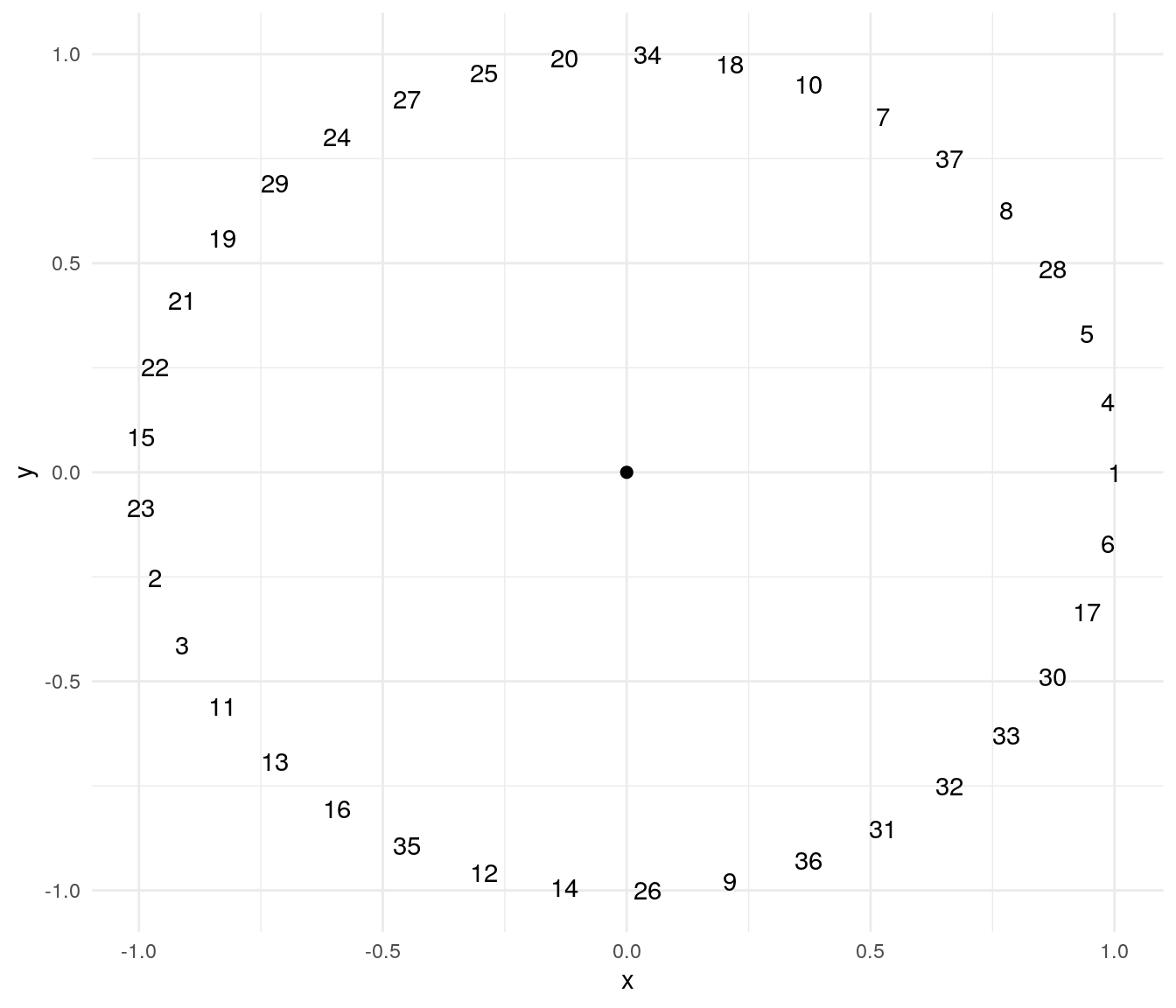
test$fit## [1] 8.216513e-05As we can see, the result is fair better than the first solution obtained.
Tracking the algorithm
I have set eval=TRUE in the run of the algorithm to examine the evolution of the obtention of the solution. Let’s plot the evolution of \(f\) and \(f^{*}\) as a function of the number of iterations. I have set a logarithmic scale in the horizontal axis, as changes in scale of the fitness function occur after the first iterations.
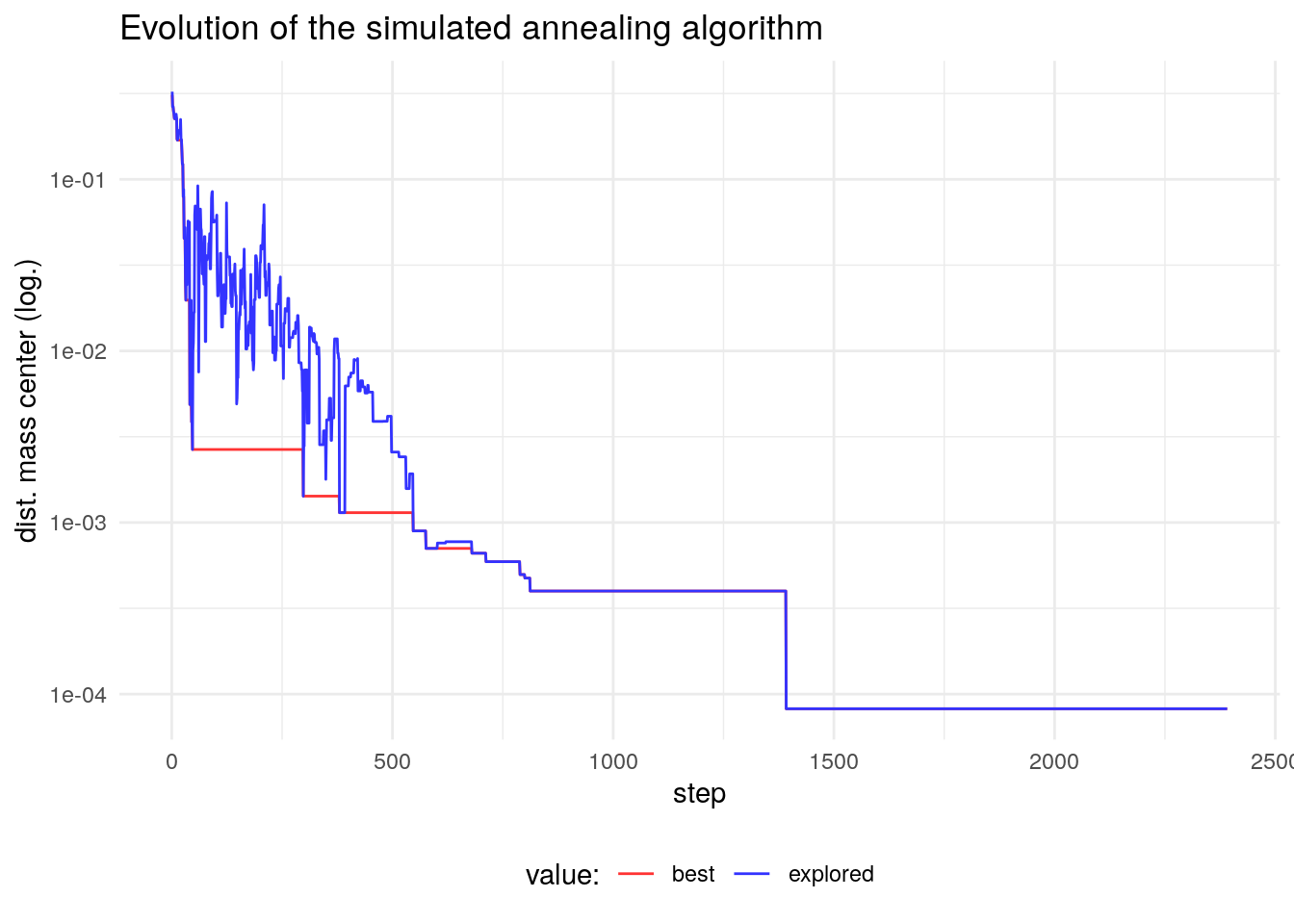
The plot shows that the algorithm is accepting values of \(f'\) with a smaller gap from \(f\) as the number of iterations increases. The simulated annealing emphasizes exploration in the first iterations, and exploitation or refinement of the solution in the last iterations.
References
- Professor Éric Taillard’s website: http://mistic.heig-vd.ch/taillard/
Session info
## R version 4.1.2 (2021-11-01)
## Platform: x86_64-pc-linux-gnu (64-bit)
## Running under: Debian GNU/Linux 10 (buster)
##
## Matrix products: default
## BLAS:   /usr/lib/x86_64-linux-gnu/blas/libblas.so.3.8.0
## LAPACK: /usr/lib/x86_64-linux-gnu/lapack/liblapack.so.3.8.0
##
## locale:
##  [1] LC_CTYPE=es_ES.UTF-8       LC_NUMERIC=C
##  [3] LC_TIME=es_ES.UTF-8        LC_COLLATE=es_ES.UTF-8
##  [5] LC_MONETARY=es_ES.UTF-8    LC_MESSAGES=es_ES.UTF-8
##  [7] LC_PAPER=es_ES.UTF-8       LC_NAME=C
##  [9] LC_ADDRESS=C               LC_TELEPHONE=C
## [11] LC_MEASUREMENT=es_ES.UTF-8 LC_IDENTIFICATION=C
##
## attached base packages:
## [1] stats     graphics  grDevices utils     datasets  methods   base
##
## other attached packages:
## [1] ggplot2_3.3.5 tidyr_1.1.4   dplyr_1.0.7
##
## loaded via a namespace (and not attached):
##  [1] highr_0.9         pillar_1.6.4      bslib_0.2.5.1     compiler_4.1.2
##  [5] jquerylib_0.1.4   tools_4.1.2       digest_0.6.27     jsonlite_1.7.2
##  [9] evaluate_0.14     lifecycle_1.0.0   tibble_3.1.5      gtable_0.3.0
## [13] pkgconfig_2.0.3   rlang_0.4.12      DBI_1.1.1         yaml_2.2.1
## [17] blogdown_1.5      xfun_0.23         withr_2.4.2       stringr_1.4.0
## [21] knitr_1.33        generics_0.1.0    vctrs_0.3.8       sass_0.4.0
## [25] grid_4.1.2        tidyselect_1.1.1  glue_1.4.2        R6_2.5.0
## [29] fansi_0.5.0       rmarkdown_2.9     bookdown_0.24     farver_2.1.0
## [33] purrr_0.3.4       magrittr_2.0.1    scales_1.1.1      ellipsis_0.3.2
## [37] htmltools_0.5.1.1 assertthat_0.2.1  colorspace_2.0-1  labeling_0.4.2
## [41] utf8_1.2.1        stringi_1.7.3     munsell_0.5.0     crayon_1.4.1