Cleaning Barcelona Air Quality Data

Jose M Sallan 2025-07-22 12 min read

The Open Data BCN portal is the official open data catalog operated by the Barcelona City Council (Ajuntament de Barcelona). It offers public data in reusable, machine‑readable formats (like CSV or JSON) across a wide range of topics, such as population, health, education, transport, economy and environment.

In this post, I will focus on the air quality data from the measure stations of the city of Barcelona, to demonstrate how the Tidyverse packages can help us to acquire and clean data from open data portals. I will also be using the clean_names() function from janitor.

library(tidyverse)
library(janitor)

Let’s pick the most recent data available about air quality. To do so, I right-click he Download button of Qualitat_Aire_Detall.csv and read it straight with read_csv().

aq_web <- read_csv("https://opendata-ajuntament.barcelona.cat/data/dataset/0582a266-ea06-4cc5-a219-913b22484e40/resource/c2032e7c-10ee-4c69-84d3-9e8caf9ca97a/download")

## Rows: 280 Columns: 57
## ── Column specification ────────────────────────────────────────────────────────
## Delimiter: ","
## chr (29): CODI_PROVINCIA, PROVINCIA, CODI_MUNICIPI, MUNICIPI, ESTACIO, V01, ...
## dbl (28): CODI_CONTAMINANT, ANY, MES, DIA, H01, H02, H03, H04, H05, H06, H07...
## 
## ℹ Use `spec()` to retrieve the full column specification for this data.
## ℹ Specify the column types or set `show_col_types = FALSE` to quiet this message.

Here is the resulting table.

aq_web

## # A tibble: 280 × 57
##    CODI_PROVINCIA PROVINCIA CODI_MUNICIPI MUNICIPI  ESTACIO CODI_CONTAMINANT
##    <chr>          <chr>     <chr>         <chr>     <chr>              <dbl>
##  1 08             Barcelona 019           Barcelona 043                  999
##  2 08             Barcelona 019           Barcelona 043                  999
##  3 08             Barcelona 019           Barcelona 043                  999
##  4 08             Barcelona 019           Barcelona 043                  999
##  5 08             Barcelona 019           Barcelona 054                  999
##  6 08             Barcelona 019           Barcelona 054                  999
##  7 08             Barcelona 019           Barcelona 054                  999
##  8 08             Barcelona 019           Barcelona 054                  999
##  9 08             Barcelona 019           Barcelona 043                   22
## 10 08             Barcelona 019           Barcelona 043                   22
## # ℹ 270 more rows
## # ℹ 51 more variables: ANY <dbl>, MES <dbl>, DIA <dbl>, H01 <dbl>, V01 <chr>,
## #   H02 <dbl>, V02 <chr>, H03 <dbl>, V03 <chr>, H04 <dbl>, V04 <chr>,
## #   H05 <dbl>, V05 <chr>, H06 <dbl>, V06 <chr>, H07 <dbl>, V07 <chr>,
## #   H08 <dbl>, V08 <chr>, H09 <dbl>, V09 <chr>, H10 <dbl>, V10 <chr>,
## #   H11 <dbl>, V11 <chr>, H12 <dbl>, V12 <chr>, H13 <dbl>, V13 <chr>,
## #   H14 <dbl>, V14 <chr>, H15 <dbl>, V15 <chr>, H16 <dbl>, V16 <chr>, …

This table is not ready to be used for a variety of reasons:

Redundant information of columns from CODI_PROVINCIA to MUNICIPI.
The VXX columns are not necessary, as they indicate that the data is missing in the corresponding HXX column.
Each row carries information of 24 hourly observations from a pollutant in a specific station. We need to reshape the data as tidy data, so each row presents information about one pollutant measured at a station at a specific hour.
We need a date time variable with the date and time when the information was obtained.

Let’s start cleaning the column names. In this case, this means that all names will be turned into small caps.

aq_web |>
  clean_names()

## # A tibble: 280 × 57
##    codi_provincia provincia codi_municipi municipi  estacio codi_contaminant
##    <chr>          <chr>     <chr>         <chr>     <chr>              <dbl>
##  1 08             Barcelona 019           Barcelona 043                  999
##  2 08             Barcelona 019           Barcelona 043                  999
##  3 08             Barcelona 019           Barcelona 043                  999
##  4 08             Barcelona 019           Barcelona 043                  999
##  5 08             Barcelona 019           Barcelona 054                  999
##  6 08             Barcelona 019           Barcelona 054                  999
##  7 08             Barcelona 019           Barcelona 054                  999
##  8 08             Barcelona 019           Barcelona 054                  999
##  9 08             Barcelona 019           Barcelona 043                   22
## 10 08             Barcelona 019           Barcelona 043                   22
## # ℹ 270 more rows
## # ℹ 51 more variables: any <dbl>, mes <dbl>, dia <dbl>, h01 <dbl>, v01 <chr>,
## #   h02 <dbl>, v02 <chr>, h03 <dbl>, v03 <chr>, h04 <dbl>, v04 <chr>,
## #   h05 <dbl>, v05 <chr>, h06 <dbl>, v06 <chr>, h07 <dbl>, v07 <chr>,
## #   h08 <dbl>, v08 <chr>, h09 <dbl>, v09 <chr>, h10 <dbl>, v10 <chr>,
## #   h11 <dbl>, v11 <chr>, h12 <dbl>, v12 <chr>, h13 <dbl>, v13 <chr>,
## #   h14 <dbl>, v14 <chr>, h15 <dbl>, v15 <chr>, h16 <dbl>, v16 <chr>, …

Then, we are ready to select the columns. Additionnally, I will put the station codes as integer numbers.

aq_web |>
  clean_names() |>
  select(c(estacio:dia, starts_with("h"))) |>
  mutate(estacio = as.numeric(estacio))

## # A tibble: 280 × 29
##    estacio codi_contaminant   any   mes   dia    h01   h02   h03   h04   h05
##      <dbl>            <dbl> <dbl> <dbl> <dbl>  <dbl> <dbl> <dbl> <dbl> <dbl>
##  1      43              999  2025     7    19   21.6  16.7  16.8  15.6  13  
##  2      43              999  2025     7    20   15.5  16.6  18.4  16    14.2
##  3      43              999  2025     7    21   28.7  19.4  18    18.3  11.6
##  4      43              999  2025     7    22   NA    NA    NA    NA    NA  
##  5      54              999  2025     7    19    9.7   8.8   6.9   9.1   9  
##  6      54              999  2025     7    20    7.5   7.8   7.7   7.8   8.4
##  7      54              999  2025     7    21   20.9  15.5  16.6  14.3  11.4
##  8      54              999  2025     7    22   26    14.8  17.3  15.1  11.8
##  9      43               22  2025     7    19  831   583   626   777   530  
## 10      43               22  2025     7    20 1123   715   689   444   419  
## # ℹ 270 more rows
## # ℹ 19 more variables: h06 <dbl>, h07 <dbl>, h08 <dbl>, h09 <dbl>, h10 <dbl>,
## #   h11 <dbl>, h12 <dbl>, h13 <dbl>, h14 <dbl>, h15 <dbl>, h16 <dbl>,
## #   h17 <dbl>, h18 <dbl>, h19 <dbl>, h20 <dbl>, h21 <dbl>, h22 <dbl>,
## #   h23 <dbl>, h24 <dbl>

And now we are ready to set the data in long format, using tidyr::pivot_longer(), Here I have used some specific settings:

The variable with column names is labelled hora (hour)-
I set names_prefix = "h" so the h is removed from column hora.
The actual value of pollutant is stored in the value column.

aq_web |>
  clean_names() |>
  select(c(estacio:dia, starts_with("h"))) |>
  mutate(estacio = as.numeric(estacio)) |>
  pivot_longer(h01:h24, names_prefix = "h", 
               names_to = "hora", values_to = "value")

## # A tibble: 6,720 × 7
##    estacio codi_contaminant   any   mes   dia hora  value
##      <dbl>            <dbl> <dbl> <dbl> <dbl> <chr> <dbl>
##  1      43              999  2025     7    19 01     21.6
##  2      43              999  2025     7    19 02     16.7
##  3      43              999  2025     7    19 03     16.8
##  4      43              999  2025     7    19 04     15.6
##  5      43              999  2025     7    19 05     13  
##  6      43              999  2025     7    19 06     21.4
##  7      43              999  2025     7    19 07     NA  
##  8      43              999  2025     7    19 08     17.7
##  9      43              999  2025     7    19 09     21.2
## 10      43              999  2025     7    19 10     15.6
## # ℹ 6,710 more rows

Finally, I generate the datetime variable with lubridate::make_datetime() and use dplyr::relocate() to place it after the codi_contaminant column.

aq_web |>
  clean_names() |>
  select(c(estacio:dia, starts_with("h"))) |>
  mutate(estacio = as.numeric(estacio)) |>
  pivot_longer(-c(estacio:dia), names_prefix = "h", 
               names_to = "hora", values_to = "value") |>
  mutate(hora = as.numeric(hora)) |>
  mutate(datetime = make_datetime(year = any, month = mes, day = dia, hour = hora)) |>
  relocate(datetime, .after = codi_contaminant)

## # A tibble: 6,720 × 8
##    estacio codi_contaminant datetime              any   mes   dia  hora value
##      <dbl>            <dbl> <dttm>              <dbl> <dbl> <dbl> <dbl> <dbl>
##  1      43              999 2025-07-19 01:00:00  2025     7    19     1  21.6
##  2      43              999 2025-07-19 02:00:00  2025     7    19     2  16.7
##  3      43              999 2025-07-19 03:00:00  2025     7    19     3  16.8
##  4      43              999 2025-07-19 04:00:00  2025     7    19     4  15.6
##  5      43              999 2025-07-19 05:00:00  2025     7    19     5  13  
##  6      43              999 2025-07-19 06:00:00  2025     7    19     6  21.4
##  7      43              999 2025-07-19 07:00:00  2025     7    19     7  NA  
##  8      43              999 2025-07-19 08:00:00  2025     7    19     8  17.7
##  9      43              999 2025-07-19 09:00:00  2025     7    19     9  21.2
## 10      43              999 2025-07-19 10:00:00  2025     7    19    10  15.6
## # ℹ 6,710 more rows

Reading several months

Now that we know how to transform a table, let’s wrap together some tables with the same structure. Right-clicking in the adequate buttons, I have obtained the links of the air quality files form January to April 2025. I have wrapped them into the links list.

ene_2025 <- "https://opendata-ajuntament.barcelona.cat/data/dataset/0582a266-ea06-4cc5-a219-913b22484e40/resource/701c14fa-e248-45c6-ac47-77384bab1670/download"
feb_2025 <- "https://opendata-ajuntament.barcelona.cat/data/dataset/0582a266-ea06-4cc5-a219-913b22484e40/resource/f0acc2d3-0657-4e57-93bd-a335ab356c9c/download"
mar_2025 <- "https://opendata-ajuntament.barcelona.cat/data/dataset/0582a266-ea06-4cc5-a219-913b22484e40/resource/04096ce5-cabd-4f66-b091-c090680c39a8/download"
abr_2025 <- "https://opendata-ajuntament.barcelona.cat/data/dataset/0582a266-ea06-4cc5-a219-913b22484e40/resource/99830447-f31f-4cbc-8c51-9c861596f644/download"

links <- list(ene_2025, feb_2025, mar_2025, abr_2025)

We can use purrr:map() to read all datasets and store them in a list.

aq_web_2025 <- map(links, read_csv)

## Rows: 2170 Columns: 57
## ── Column specification ────────────────────────────────────────────────────────
## Delimiter: ","
## chr (26): PROVINCIA, MUNICIPI, V01, V02, V03, V04, V05, V06, V07, V08, V09, ...
## dbl (31): CODI_PROVINCIA, CODI_MUNICIPI, ESTACIO, CODI_CONTAMINANT, ANY, MES...
## 
## ℹ Use `spec()` to retrieve the full column specification for this data.
## ℹ Specify the column types or set `show_col_types = FALSE` to quiet this message.
## Rows: 1960 Columns: 57
## ── Column specification ────────────────────────────────────────────────────────
## Delimiter: ","
## chr (26): PROVINCIA, MUNICIPI, V01, V02, V03, V04, V05, V06, V07, V08, V09, ...
## dbl (31): CODI_PROVINCIA, CODI_MUNICIPI, ESTACIO, CODI_CONTAMINANT, ANY, MES...
## 
## ℹ Use `spec()` to retrieve the full column specification for this data.
## ℹ Specify the column types or set `show_col_types = FALSE` to quiet this message.
## Rows: 2170 Columns: 57
## ── Column specification ────────────────────────────────────────────────────────
## Delimiter: ","
## chr (26): PROVINCIA, MUNICIPI, V01, V02, V03, V04, V05, V06, V07, V08, V09, ...
## dbl (31): CODI_PROVINCIA, CODI_MUNICIPI, ESTACIO, CODI_CONTAMINANT, ANY, MES...
## 
## ℹ Use `spec()` to retrieve the full column specification for this data.
## ℹ Specify the column types or set `show_col_types = FALSE` to quiet this message.
## Rows: 2030 Columns: 57
## ── Column specification ────────────────────────────────────────────────────────
## Delimiter: ","
## chr (26): PROVINCIA, MUNICIPI, V01, V02, V03, V04, V05, V06, V07, V08, V09, ...
## dbl (31): CODI_PROVINCIA, CODI_MUNICIPI, ESTACIO, CODI_CONTAMINANT, ANY, MES...
## 
## ℹ Use `spec()` to retrieve the full column specification for this data.
## ℹ Specify the column types or set `show_col_types = FALSE` to quiet this message.

Now I am wrapping into a clean_aq_table() all the steps to clean each of the tables.

clean_aq_table <- function(table){
  t <- table |>
  clean_names() |>
  select(c(estacio:dia, starts_with("h"))) |>
  mutate(estacio = as.numeric(estacio)) |>
  pivot_longer(-c(estacio:dia), names_prefix = "h", 
               names_to = "hora", values_to = "value") |>
  mutate(hora = as.numeric(hora)) |>
  mutate(datetime = make_datetime(year = any, month = mes, day = dia, hour = hora)) |>
  relocate(datetime, .after = codi_contaminant)
  
  return(t)
}

I am using purrr:map_dfr() to clean each element of the aq_web_2025 list and to bind the rows of all the tables.

aq_tidy_2025 <- map_dfr(aq_web_2025, clean_aq_table)

Here is the result: a tidy table of air quality data of the first four months of 2025.

aq_tidy_2025

## # A tibble: 199,920 × 8
##    estacio codi_contaminant datetime              any   mes   dia  hora value
##      <dbl>            <dbl> <dttm>              <dbl> <dbl> <dbl> <dbl> <dbl>
##  1       4                7 2025-01-01 01:00:00  2025     1     1     1    13
##  2       4                7 2025-01-01 02:00:00  2025     1     1     2    11
##  3       4                7 2025-01-01 03:00:00  2025     1     1     3     9
##  4       4                7 2025-01-01 04:00:00  2025     1     1     4     7
##  5       4                7 2025-01-01 05:00:00  2025     1     1     5     1
##  6       4                7 2025-01-01 06:00:00  2025     1     1     6     2
##  7       4                7 2025-01-01 07:00:00  2025     1     1     7     1
##  8       4                7 2025-01-01 08:00:00  2025     1     1     8     1
##  9       4                7 2025-01-01 09:00:00  2025     1     1     9     1
## 10       4                7 2025-01-01 10:00:00  2025     1     1    10     2
## # ℹ 199,910 more rows

Examining the Dataset

Now that it is in tidy format, it is easy to examine the data in several ways. For instance, we can check at what dates and stations the daily average value of PM10 codi_contaminant == 10 where higher than 50 µg/m³.

aq_tidy_2025 |>
  filter(codi_contaminant == 10) |>
  mutate(date = as_date(datetime)) |>
  group_by(estacio, date) |>
  summarise(mean_pm10 = mean(value, na.rm = TRUE), .groups = "drop") |>
  arrange(-mean_pm10)

## # A tibble: 720 × 3
##    estacio date       mean_pm10
##      <dbl> <date>         <dbl>
##  1      43 2025-01-22      42.6
##  2      43 2025-03-21      39.5
##  3       4 2025-03-21      38.5
##  4      43 2025-02-05      38.3
##  5      43 2025-01-20      37.5
##  6      57 2025-02-05      37  
##  7      57 2025-04-14      36.8
##  8      57 2025-02-17      36.7
##  9      54 2025-02-06      36.5
## 10      43 2025-02-06      36.5
## # ℹ 710 more rows

As the highest value of daily average of PM10 is smaller than 50, no episodes of pollution caused by PM10 were caused by this pollutant.

As station 43 (Eixample) seems to have the highest values of PM10, let’s plot the average daily value of PM10 with a line plot.

aq_tidy_2025 |>
  filter(codi_contaminant == 10, estacio == 43) |>
  mutate(date = as_date(datetime)) |>
  group_by(date) |>
  summarise(mean_pm10 = mean(value, na.rm = TRUE)) |>
  ggplot(aes(date, mean_pm10)) +
  geom_line() +
    theme_minimal() +
  labs(title = "Daily values of PM10 at the Eixample station", x= NULL, y = NULL)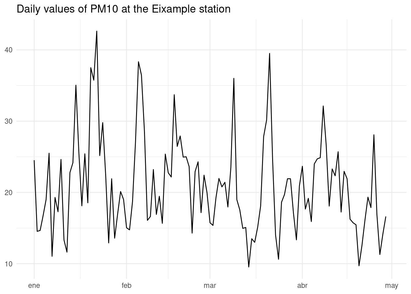

Open Data with R

Open data portals are a valuable source of data of the city life, from commercial activity to air quality. The R environment, specially the Tidyverse, offers a good platform to clean and structure the data for analysis effectively. A second step in this process is to retrieve the data more effectively than right-clicking in the web. This is quite platform specific and requires examining the information for developers of the portal.

References

Air quality data from the measure stations of the city of Barcelona https://opendata-ajuntament.barcelona.cat/data/en/dataset/qualitat-aire-detall-bcn
Air quality measure stations of the city of Barcelona https://opendata-ajuntament.barcelona.cat/data/en/dataset/qualitat-aire-estacions-bcn
Measured air pollutants by the air quality measurement stations of the city of Barcelona https://opendata-ajuntament.barcelona.cat/data/en/dataset/contaminants-estacions-mesura-qualitat-aire

All websites checked on 22 July 2025.

Session Info

## R version 4.5.1 (2025-06-13)
## Platform: x86_64-pc-linux-gnu
## Running under: Linux Mint 21.1
## 
## Matrix products: default
## BLAS:   /usr/lib/x86_64-linux-gnu/blas/libblas.so.3.10.0 
## LAPACK: /usr/lib/x86_64-linux-gnu/lapack/liblapack.so.3.10.0  LAPACK version 3.10.0
## 
## locale:
##  [1] LC_CTYPE=es_ES.UTF-8       LC_NUMERIC=C              
##  [3] LC_TIME=es_ES.UTF-8        LC_COLLATE=es_ES.UTF-8    
##  [5] LC_MONETARY=es_ES.UTF-8    LC_MESSAGES=es_ES.UTF-8   
##  [7] LC_PAPER=es_ES.UTF-8       LC_NAME=C                 
##  [9] LC_ADDRESS=C               LC_TELEPHONE=C            
## [11] LC_MEASUREMENT=es_ES.UTF-8 LC_IDENTIFICATION=C       
## 
## time zone: Europe/Madrid
## tzcode source: system (glibc)
## 
## attached base packages:
## [1] stats     graphics  grDevices utils     datasets  methods   base     
## 
## other attached packages:
##  [1] janitor_2.2.1   lubridate_1.9.4 forcats_1.0.0   stringr_1.5.1  
##  [5] dplyr_1.1.4     purrr_1.0.4     readr_2.1.5     tidyr_1.3.1    
##  [9] tibble_3.2.1    ggplot2_3.5.2   tidyverse_2.0.0
## 
## loaded via a namespace (and not attached):
##  [1] utf8_1.2.4        sass_0.4.10       generics_0.1.3    blogdown_1.21    
##  [5] stringi_1.8.7     hms_1.1.3         digest_0.6.37     magrittr_2.0.3   
##  [9] evaluate_1.0.3    grid_4.5.1        timechange_0.3.0  bookdown_0.43    
## [13] fastmap_1.2.0     jsonlite_2.0.0    scales_1.3.0      jquerylib_0.1.4  
## [17] cli_3.6.4         rlang_1.1.6       crayon_1.5.3      bit64_4.6.0-1    
## [21] munsell_0.5.1     withr_3.0.2       cachem_1.1.0      yaml_2.3.10      
## [25] tools_4.5.1       parallel_4.5.1    tzdb_0.5.0        colorspace_2.1-1 
## [29] curl_6.2.2        vctrs_0.6.5       R6_2.6.1          lifecycle_1.0.4  
## [33] snakecase_0.11.1  bit_4.6.0         vroom_1.6.5       pkgconfig_2.0.3  
## [37] pillar_1.10.2     bslib_0.9.0       gtable_0.3.6      glue_1.8.0       
## [41] xfun_0.52         tidyselect_1.2.1  rstudioapi_0.17.1 knitr_1.50       
## [45] farver_2.1.2      htmltools_0.5.8.1 labeling_0.4.3    rmarkdown_2.29   
## [49] compiler_4.5.1

The Jose M Sallan static website