In this post, I will make a short introduction to decision trees for classification problems with the C50 package, a R wrapper for the C5.0 algorithm (Quinlan, 1993). I will also use the dplyr and ggplot2 for data manipulation and visualization, BAdatasets to access the WineQuality dataset and yardstick to obtain classification metrics.
library(dplyr)
library(ggplot2)
library(C50)
library(BAdatasets)
library(yardstick)
The approach of decision trees to prediction consists of using the features to divide data into smaller and smaller groups, so that in each group most of the observations belong to the same category of the target variable. We use features to build a decision tree through recursive partitioning. It starts including all training data in a root node, and splitting data into two subsets according to the values of a feature. This process is repeated for different nodes creating a tree-like structure, whose terminal nodes are called leaves. Elements falling in a leaf will be assigned the class of the majority of elements of the leaf. This process can have several stopping criteria:
- the observations of each leaf have a majority of elements of the same class.
- the number of elements in each leaf reaches a minimal value.
- the tree has grown into a size limit.
Decision trees can also be presented as sets of if-then statements called decision rules. The if term contains a logical operator based on a combination of feature values, and the then assigns elements for which the statement is true to a class.
Let’s start exploring C50 with a set of synthetic data s_data:
n <- 400
set.seed(2020)
x <- c(runif(n*0.5, 0, 10), runif(n*0.25, 4, 10), runif(n*0.25, 0, 6))
y <- c(runif(n*0.5, 0, 5), runif(n*0.25, 4, 10), runif(n*0.25, 4, 10))
class <- as.factor(c(rep("a", n*0.5), c(rep("b", n*0.25)), c(rep("c", n*0.25))))

s_data <- tibble(x=x, y=y, class = class)

s_data %>%
  ggplot(aes(x, y, col=class)) +
  geom_point() +
  theme_minimal()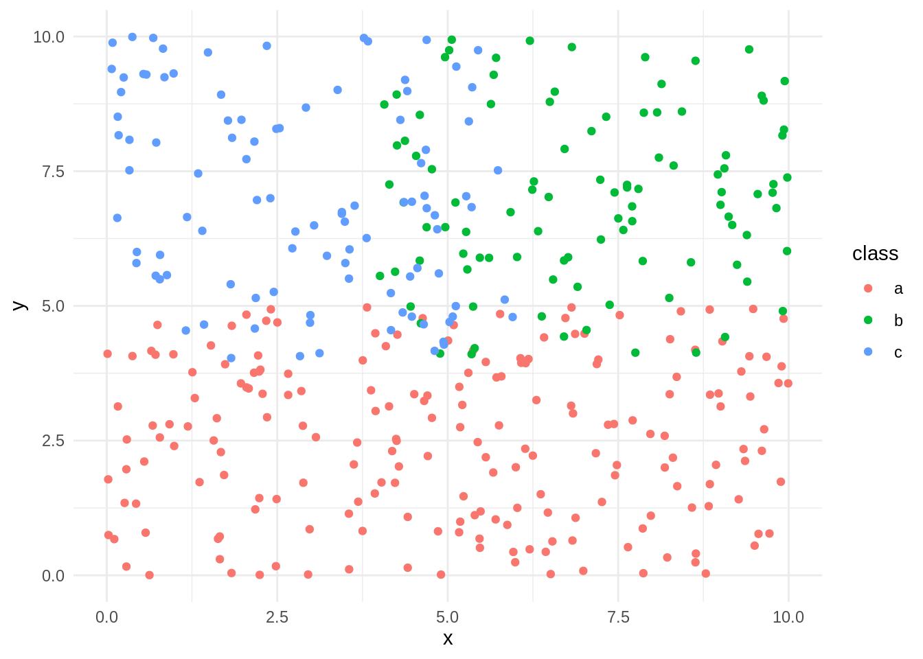
The task is to predict the value of class based on the features x and y. I use the C5.0 function with formula and data as arguments and setting rules=FALSE to obtain a decision tree.
dt <- C5.0(class ~ ., data = s_data, rules=FALSE)
summary(dt)
##
## Call:
## C5.0.formula(formula = class ~ ., data = s_data, rules = FALSE)
##
##
## C5.0 [Release 2.07 GPL Edition] Mon Jul 11 11:53:23 2022
## -------------------------------
##
## Class specified by attribute `outcome'
##
## Read 400 cases (3 attributes) from undefined.data
##
## Decision tree:
##
## y <= 4.972004: a (229/29)
## y > 4.972004:
## :...x <= 3.875929: c (57)
## x > 3.875929: b (114/25)
##
##
## Evaluation on training data (400 cases):
##
## Decision Tree
## ----------------
## Size Errors
##
## 3 54(13.5%) <<
##
##
## (a) (b) (c) <-classified as
## ---- ---- ----
## 200 (a): class a
## 11 89 (b): class b
## 18 25 57 (c): class c
##
##
## Attribute usage:
##
## 100.00% y
## 42.75% x
##
##
## Time: 0.0 secsC50 has a plot method for decision trees:
plot(dt)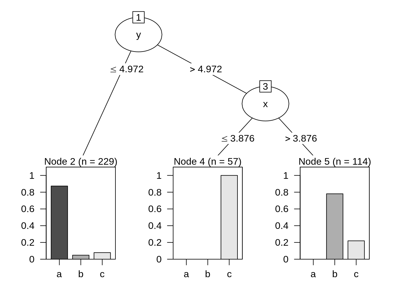
From this plot we learn how the algorithm works: first it splits node 1 into nodes 2 and 3 based on the value of y. Then, it splits node 3 based on the value of x. Observations in node 2 will be labelled with class a, observations in node 3 to class c and observations in node 5 to class b.
The plot help us to interpret some information obtained in the summary:
- The tree has classified incorrectly 54 out of 400 observations, the 13.5% of total. This means that the accuracy of this classification is equal to 100% - 13.5% = 86.50%.
- All observations of class a have been classified correctly, while 11 observations of class
band 18 + 25 = 43 ofchave been classified incorrectly. This can be seen in theEvaluation of training datasection of the summary. - Feature
yhas been used to classify all observations, whilexhas been used only for observations in leaves 4 and 5. In theAttribute usagesection of the summary we see thatyhas a variable importance of 100% andxonly of 42.75%, the proportion of observations in leaves 4 and 5.
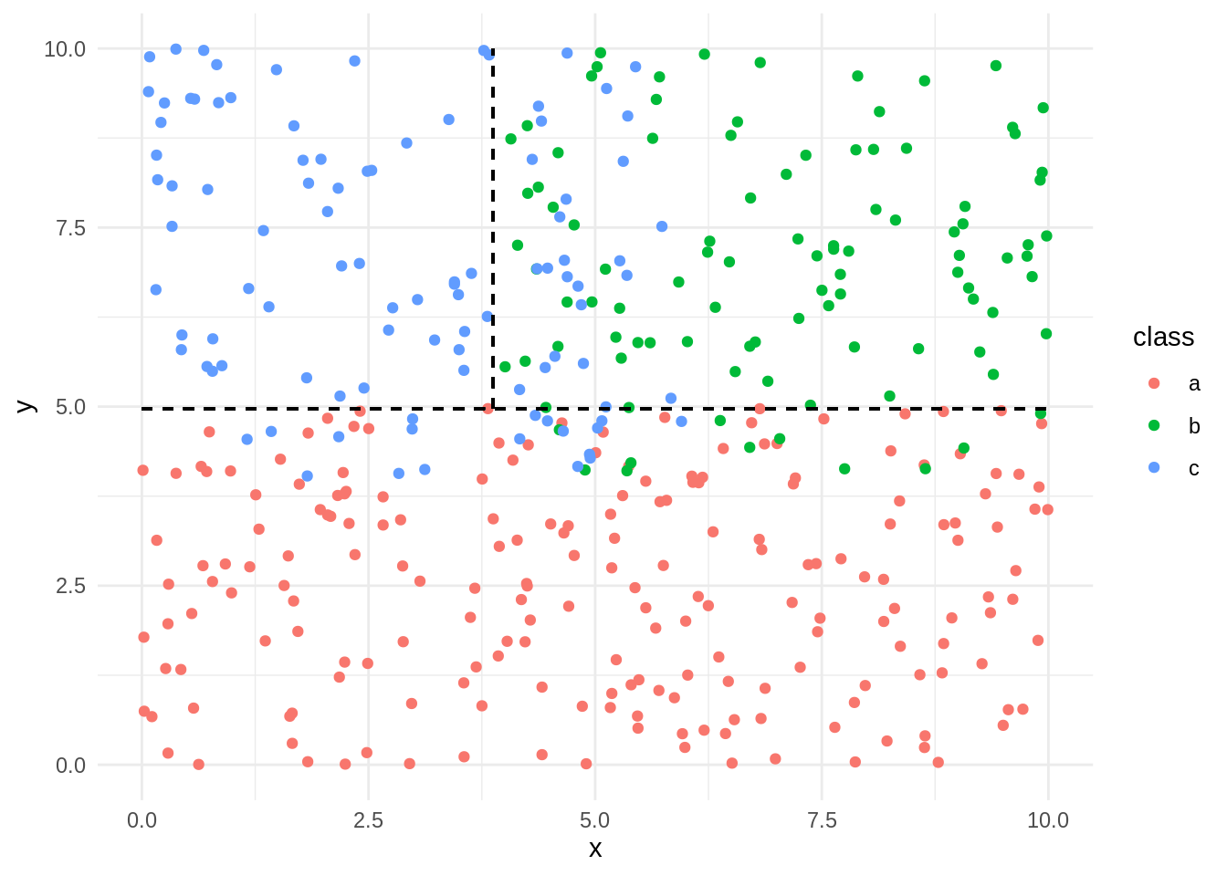
Here is an alternative representation of the classification in the original scatter plot:
If we set rules=TRUE we obtain the classification as a set of rules equivalent to the decision tree:
dr <- C5.0(class ~ ., data = s_data, rules=TRUE)
summary(dr)
##
## Call:
## C5.0.formula(formula = class ~ ., data = s_data, rules = TRUE)
##
##
## C5.0 [Release 2.07 GPL Edition] Mon Jul 11 11:53:24 2022
## -------------------------------
##
## Class specified by attribute `outcome'
##
## Read 400 cases (3 attributes) from undefined.data
##
## Rules:
##
## Rule 1: (229/29, lift 1.7)
## y <= 4.972004
## -> class a [0.870]
##
## Rule 2: (114/25, lift 3.1)
## x > 3.875929
## y > 4.972004
## -> class b [0.776]
##
## Rule 3: (57, lift 3.9)
## x <= 3.875929
## y > 4.972004
## -> class c [0.983]
##
## Default class: a
##
##
## Evaluation on training data (400 cases):
##
## Rules
## ----------------
## No Errors
##
## 3 54(13.5%) <<
##
##
## (a) (b) (c) <-classified as
## ---- ---- ----
## 200 (a): class a
## 11 89 (b): class b
## 18 25 57 (c): class c
##
##
## Attribute usage:
##
## 100.00% y
## 42.75% x
##
##
## Time: 0.0 secsClassifying the Wine Quality data set with C50
Let’s test the algorithm with a more complex example, WineQuality. It consists of two datasets with chemical properties of red and white vinho verde samples from the north of Portugal. I will be merging both datasets into one adding a type variable to distinguish red and white wines.
data("WineQuality")

red <- WineQuality$red %>%
  mutate(type = "red")
white <- WineQuality$white %>%
  mutate(type = "white")

wines <- bind_rows(red, white) %>%
  mutate(type = factor(type))
The target variable is quality, which has several categories:
wines %>%
  ggplot(aes(factor(quality))) +
  geom_bar() +
  theme_minimal()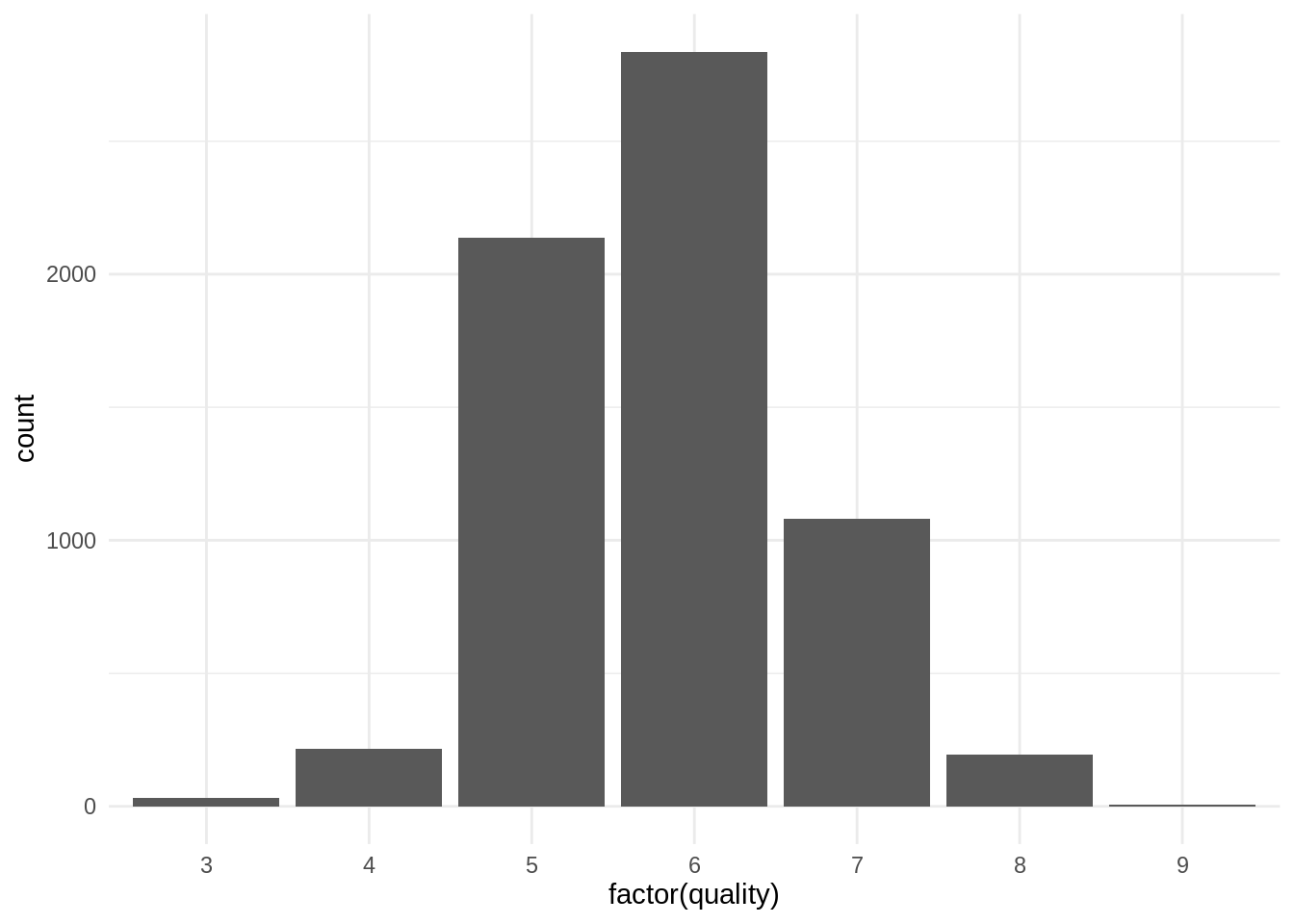
We have a too small number of observations for values of quality equal to three and 9, so I will collapse quality 3 into 4 and quality 9 into 8, respectively.
wines <- wines %>%
  mutate(quality = case_when(quality == 3 ~ 4,
                             quality == 9 ~ 8,
                             !quality %in% c(3,9) ~ quality))
wines <- wines %>%
  mutate(quality = factor(quality))
Now we have values of quality from 4 to 8:
wines %>%
  ggplot(aes(quality)) +
  geom_bar() +
  theme_minimal()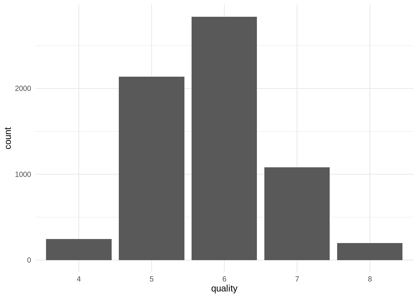
Let’s build a decision tree on the dataset.
wine_dt <- C5.0(quality ~ ., data = wines)Winnowing and boosting
The C5.0 algorithm has two additional features to improve classificaation performance:
- select which features include in the analysis through winnowing.
- boosting the weight of some observations.
Winnowing consists of pre-selecting a subset of the attributes that will be used to construct the decision tree. According to the developers of the algorithm, it can be useful for situations where some of the attributes have at best marginal relevance to the classification task. We apply winnowing to the classifyer making winnow=TRUE.
When using boosting, C5.0 produces several decision trees iteratively:
- We obtain an initial decision tree applying the C5.0 algorithm.
- The algorithm detects the observations that have not been classified correctly, and increases their weight to compute node purity.
- A new decision tree is obtained using the weights obtained above.
- Boosting stops when the obtained classifier is highly accurate or too inaccurate, or when a number of trials is reached.
We can use boosting in C5.0 setting a value of trials larger than one.
Let’s obtain a new decision tree applying winnowing and boosting.
wine_dt_winnow <- C5.0(quality ~ ., data = wines,
                       winnow = TRUE,
                       trials = 5)
Comparing performance
I will use the yardstick package from tidymodels to obtain performance parameters of the two classifiers:
- I am using the
predictmethod for each decision tree, and store real and predicted values into aclass_winestibble. - I am defining a metric set
class_metricsincluding accuracy, precision and recall.
Let’s remember that:
- accuracy is the fraction of observations classified correctly.
- precision is the fraction of observations that have been assigned a category classified correctly. It is averaged across categories.
- recall is the fraction of observations belonging to a category classified correctly. It is also averaged across categories.
class_wines <- tibble(value = wines$quality,
                      predict = predict(wine_dt, wines),
                      predict_w = predict(wine_dt_winnow, wines))

class_metrics <- metric_set(accuracy, precision, recall)
Let’s examine the confusion matrix for the two decision trees:
conf_mat(class_wines, truth = value, estimate = predict)## Truth
## Prediction 4 5 6 7 8
## 4 152 12 5 4 1
## 5 56 1719 232 26 6
## 6 36 372 2415 180 25
## 7 2 33 175 864 52
## 8 0 2 9 5 114class_metrics(class_wines, truth = value, estimate = predict)## # A tibble: 3 × 3
## .metric .estimator .estimate
## <chr> <chr> <dbl>
## 1 accuracy multiclass 0.810
## 2 precision macro 0.832
## 3 recall macro 0.730And the performance metrics:
conf_mat(class_wines, truth = value, estimate = predict_w)## Truth
## Prediction 4 5 6 7 8
## 4 175 2 0 0 0
## 5 50 2019 155 11 4
## 6 20 108 2657 109 13
## 7 1 8 21 957 12
## 8 0 1 3 2 169class_metrics(class_wines, truth = value, estimate = predict_w)## # A tibble: 3 × 3
## .metric .estimator .estimate
## <chr> <chr> <dbl>
## 1 accuracy multiclass 0.920
## 2 precision macro 0.946
## 3 recall macro 0.867The metrics of the model with winnowing and boosting are better than the ones of the baseline model. As I have not split the dataset into train and test, I cannot control if the obtained classifiers overfit to the train test.
Variable importance
We can learn about which variables are more relevant in a decision tree with variable importance. In the C50 package, the importance of a variable is equal to the proportion of observations that have been classified using that variable. For instance, the variable used in the first split has an importance of 100%.
In the summary of a call to C5.0, the importance of variables is in the Attribute usage section. We can obtain these values with C5imp:
C5imp(wine_dt)## Overall
## volatileacidity 100.00
## alcohol 100.00
## freesulfurdioxide 83.45
## fixedacidity 72.66
## sulphates 67.18
## citricacid 60.63
## pH 51.44
## residualsugar 49.87
## totalsulfurdioxide 47.05
## chlorides 44.13
## density 41.34
## type 37.31
## fixed acidity 0.00
## volatile acidity 0.00
## citric acid 0.00
## residual sugar 0.00
## free sulfur dioxide 0.00
## total sulfur dioxide 0.00The same values for the classification with winnowing and boosting.
C5imp(wine_dt_winnow)## Overall
## volatileacidity 100.00
## alcohol 100.00
## freesulfurdioxide 99.80
## sulphates 99.03
## fixedacidity 99.00
## citricacid 97.44
## pH 95.74
## totalsulfurdioxide 94.95
## chlorides 93.58
## residualsugar 93.47
## density 83.01
## type 78.93
## fixed acidity 0.00
## volatile acidity 0.00
## citric acid 0.00
## residual sugar 0.00
## free sulfur dioxide 0.00
## total sulfur dioxide 0.00The C50 implements in R the C5.0 classification model described in Quinlan (1993). It can be used only for classification problems, although it includes feature selection with winnowing and boosting of anomalous observations using cross validation.
References
- C5.0 Classification Models https://cran.r-project.org/web/packages/C50/vignettes/C5.0.html
- Kuhn, M., & Johnson, K. (2013). Applied predictive modeling. New York: Springer. Cortez, P et al. (2009). Wine Quality Data Set. https://archive.ics.uci.edu/ml/datasets/wine+quality
- Quinlan, J. R. (1993). C4. 5: programs for machine learning. Elsevier.
- Rulequest (2019). C5.0: An Informal Tutorial. https://www.rulequest.com/see5-unix.html
Session info
## R version 4.2.0 (2022-04-22)
## Platform: x86_64-pc-linux-gnu (64-bit)
## Running under: Linux Mint 19.2
##
## Matrix products: default
## BLAS:   /usr/lib/x86_64-linux-gnu/openblas/libblas.so.3
## LAPACK: /usr/lib/x86_64-linux-gnu/libopenblasp-r0.2.20.so
##
## locale:
##  [1] LC_CTYPE=es_ES.UTF-8       LC_NUMERIC=C
##  [3] LC_TIME=es_ES.UTF-8        LC_COLLATE=es_ES.UTF-8
##  [5] LC_MONETARY=es_ES.UTF-8    LC_MESSAGES=es_ES.UTF-8
##  [7] LC_PAPER=es_ES.UTF-8       LC_NAME=C
##  [9] LC_ADDRESS=C               LC_TELEPHONE=C
## [11] LC_MEASUREMENT=es_ES.UTF-8 LC_IDENTIFICATION=C
##
## attached base packages:
## [1] stats     graphics  grDevices utils     datasets  methods   base
##
## other attached packages:
## [1] yardstick_0.0.9  BAdatasets_0.1.0 C50_0.1.6        ggplot2_3.3.5
## [5] dplyr_1.0.9
##
## loaded via a namespace (and not attached):
##  [1] tidyselect_1.1.2 xfun_0.30        bslib_0.3.1      inum_1.0-4
##  [5] purrr_0.3.4      reshape2_1.4.4   splines_4.2.0    lattice_0.20-45
##  [9] Cubist_0.4.0     colorspace_2.0-3 vctrs_0.4.1      generics_0.1.2
## [13] htmltools_0.5.2  yaml_2.3.5       utf8_1.2.2       survival_3.2-13
## [17] rlang_1.0.2      jquerylib_0.1.4  pillar_1.7.0     glue_1.6.2
## [21] withr_2.5.0      DBI_1.1.2        lifecycle_1.0.1  plyr_1.8.7
## [25] stringr_1.4.0    munsell_0.5.0    blogdown_1.9     gtable_0.3.0
## [29] mvtnorm_1.1-3    evaluate_0.15    labeling_0.4.2   knitr_1.39
## [33] fastmap_1.1.0    fansi_1.0.3      highr_0.9        Rcpp_1.0.8.3
## [37] scales_1.2.0     jsonlite_1.8.0   farver_2.1.0     digest_0.6.29
## [41] stringi_1.7.6    bookdown_0.26    grid_4.2.0       cli_3.3.0
## [45] tools_4.2.0      magrittr_2.0.3   sass_0.4.1       tibble_3.1.6
## [49] Formula_1.2-4    crayon_1.5.1     pkgconfig_2.0.3  partykit_1.2-16
## [53] ellipsis_0.3.2   libcoin_1.0-9    Matrix_1.4-1     pROC_1.18.0
## [57] assertthat_0.2.1 rmarkdown_2.14   rstudioapi_0.13  rpart_4.1.16
## [61] R6_2.5.1         compiler_4.2.0