In this post, I will introduce how to add categorical and ordinal variables to a linear regression model. I will use dplyr and ggplot2 for data handling and visualization, and kableExtra to present HTML tables. I will also present how to plot error bars with ggplot2.
library(dplyr)
library(ggplot2)
library(kableExtra)
A categorical variable can take only a limited and usually fixed set of values. Each of these values is a category. An example of categorical variable is the Species variable of the iris database, which represents the species that each observation belongs to. It can take three values: setosa, versicolor and virginica.
An ordinal variable is a categorical variable whose categories can be ordered. The dose variable of the ToothGrowth is the dose of Vitamin C administered to each Guinea pig of the sample. It can take three values: 0.5, 1 and 2.
Categorical and ordinal variables can be encoded in R as factor variables. That’s how Species is encoded in iris.
str(iris)## 'data.frame': 150 obs. of 5 variables:
## $ Sepal.Length: num 5.1 4.9 4.7 4.6 5 5.4 4.6 5 4.4 4.9 ...
## $ Sepal.Width : num 3.5 3 3.2 3.1 3.6 3.9 3.4 3.4 2.9 3.1 ...
## $ Petal.Length: num 1.4 1.4 1.3 1.5 1.4 1.7 1.4 1.5 1.4 1.5 ...
## $ Petal.Width : num 0.2 0.2 0.2 0.2 0.2 0.4 0.3 0.2 0.2 0.1 ...
## $ Species : Factor w/ 3 levels "setosa","versicolor",..: 1 1 1 1 1 1 1 1 1 1 ...We can use the levels function to obtain the categories or levels of a factor:
levels(iris$Species)## [1] "setosa" "versicolor" "virginica"The dose variable of ToothGrowth is encoded as numeric. We can transform it to ordinal doing:
ToothGrowth <- ToothGrowth %>%
  mutate(dose = as.factor(dose))
Let’s see the levels of dose:
levels(ToothGrowth$dose)## [1] "0.5" "1" "2"Dummy variables
In linear regression, we want to examine the relationship between one dependent variable and a set of independent variables. The dependent variable must be quantitative, but we can use categorical and ordinal variables as dependent variables too. To to that we need to create a binary variable for each category minus one. These variables are called dummy variables and the process of generating them one hot encoding. Let’s see the dummy variables for Species:
| species | versicolor | virginica |
|---|---|---|
| versicolor | 1 | 0 |
| virginica | 0 | 1 |
We are not defining a third dummy variable for setosa because it could be obtained as 1 - versicolor - virginica. For this encoding, setosa is the baseline level or category.
Let’s examine how the variable Sepal.Length of iris is affected by Species. We can do that with a boxplot:
ggplot(iris, aes(Species, Sepal.Length)) +
  geom_boxplot() +
  labs(title = "Values of Sepal.Length for each Species")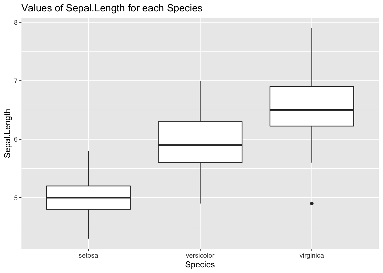
Or by comparing the 95% confidence intervals for the mean, using the mean_se function. This function returns three values: the sample mean, and the upper amd lower bound of a confidence interval obtained from the standard error, the standard deviation of the mean. I have set mult = 1.96 to obtain the 95% confidence interval. Note the wawing notation to define the ci function, introduced since R 4.0.0.
ci <- \(x) mean_se(x, mult = 1.96)
ggplot(iris, aes(Species, Sepal.Length)) +
  stat_summary(fun.data = ci) +
  labs(title = "95% confidence intervals for the mean")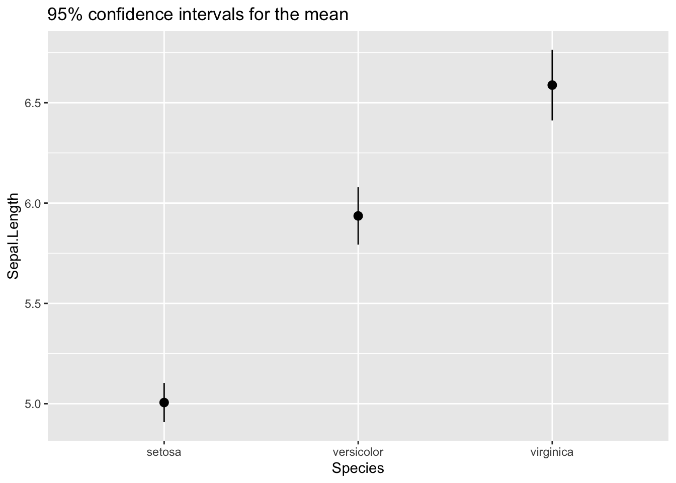
We can also draw an error bar plot, defining an iris_summary table of statistics. Using that table, I have plotted the bars with geom_bar and the CI intervals with geom_errorbar.
iris_summary <- iris %>% group_by(Species) %>%
  summarise(y=mean(Sepal.Length), sd = sd(Sepal.Length)) %>%
  mutate(ymin = y - 1.96*sd/sqrt(50), ymax = y + 1.96*sd/sqrt(50))
ggplot(iris_summary, aes(Species, y)) +
  geom_bar(stat = "identity", fill = "#8FBC8F") +
  geom_errorbar(aes(ymin = ymin, ymax = ymax), width = 0.2) +
  labs(title = "Error bars with 95% CI for the mean", y = "Sepal.Length")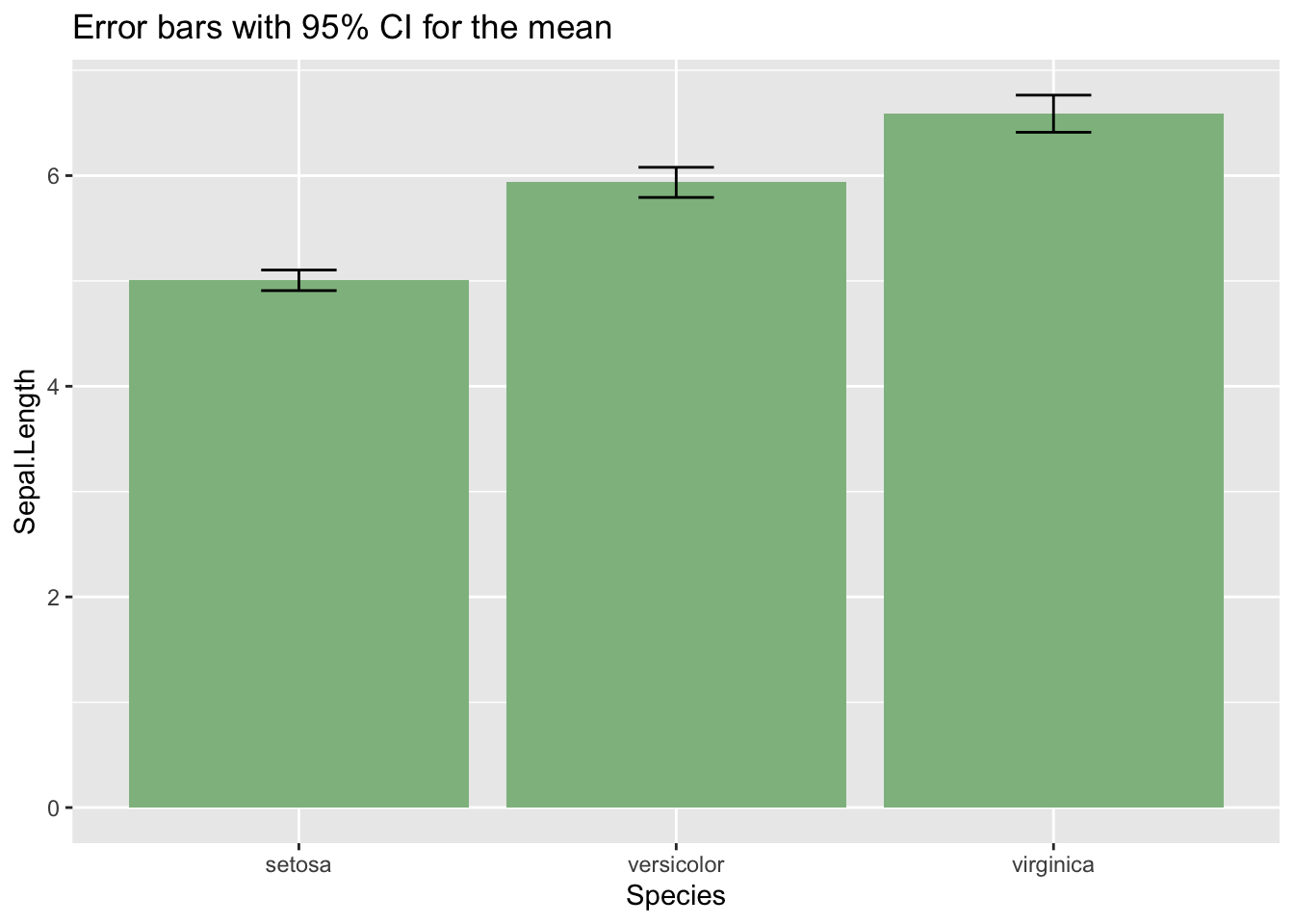
The three plots show that the mean of Sepal.Length is affected by Species. If we want to examine this using linear regression, we should define the two dummy variables described above. But we don’t need to do that if we use R: if we set a factor as a dependent variable, R generates the dummy variables, taking the first level of the factor as baseline.
m1 <- lm(Sepal.Length ~ Species, data = iris)
summary(m1)
##
## Call:
## lm(formula = Sepal.Length ~ Species, data = iris)
##
## Residuals:
## Min 1Q Median 3Q Max
## -1.6880 -0.3285 -0.0060 0.3120 1.3120
##
## Coefficients:
## Estimate Std. Error t value Pr(>|t|)
## (Intercept) 5.0060 0.0728 68.762 < 2e-16 ***
## Speciesversicolor 0.9300 0.1030 9.033 8.77e-16 ***
## Speciesvirginica 1.5820 0.1030 15.366 < 2e-16 ***
## ---
## Signif. codes: 0 '***' 0.001 '**' 0.01 '*' 0.05 '.' 0.1 ' ' 1
##
## Residual standard error: 0.5148 on 147 degrees of freedom
## Multiple R-squared: 0.6187, Adjusted R-squared: 0.6135
## F-statistic: 119.3 on 2 and 147 DF, p-value: < 2.2e-16The two dummy variables are presented as Speciesversicolor and Speciesvirginica. The regression coefficients of the dummy variables represent the difference of the mean of the dependent variable between observations from the baseline category and the category represented by each dummy variable. Here we learn that the mean of Sepal.Length of versicolor is the mean of setosa plus 0.93, and that the mean of virginica the mean of setosa plus 1.58. This is congruent with the values we observe in the error bar plot. Both regression coefficients appear to be significantly different from zero, as their p-values (in the Pr(>|t|) column) are very close to zero.
Just for checking, let’s see what happens if we make versicolor the baseline category. We can achieve that with relevel:
iris_relevel <- iris %>%
  mutate(Species = relevel(Species, "versicolor"))
Let’s estimate the new model:
m1b <- lm(Sepal.Length ~ Species, data = iris_relevel)
summary(m1b)
##
## Call:
## lm(formula = Sepal.Length ~ Species, data = iris_relevel)
##
## Residuals:
## Min 1Q Median 3Q Max
## -1.6880 -0.3285 -0.0060 0.3120 1.3120
##
## Coefficients:
## Estimate Std. Error t value Pr(>|t|)
## (Intercept) 5.9360 0.0728 81.536 < 2e-16 ***
## Speciessetosa -0.9300 0.1030 -9.033 8.77e-16 ***
## Speciesvirginica 0.6520 0.1030 6.333 2.77e-09 ***
## ---
## Signif. codes: 0 '***' 0.001 '**' 0.01 '*' 0.05 '.' 0.1 ' ' 1
##
## Residual standard error: 0.5148 on 147 degrees of freedom
## Multiple R-squared: 0.6187, Adjusted R-squared: 0.6135
## F-statistic: 119.3 on 2 and 147 DF, p-value: < 2.2e-16Now the dummy variables are Speciessetosa and Speciesvirginica. From the regression coefficients, now we observe that for setosa the mean of Sepal.Length for setosa is the mean of versicolor minus 0.93, and that the mean of virginica is equal to the mean of versicolor plus 0.65. Again, this is congruent with the results of the error bar plot.
A model with categorical and ordinal variables
Let’s move now to ToothGrowth:
str(ToothGrowth)## 'data.frame': 60 obs. of 3 variables:
## $ len : num 4.2 11.5 7.3 5.8 6.4 10 11.2 11.2 5.2 7 ...
## $ supp: Factor w/ 2 levels "OJ","VC": 2 2 2 2 2 2 2 2 2 2 ...
## $ dose: Factor w/ 3 levels "0.5","1","2": 1 1 1 1 1 1 1 1 1 1 ...The variables of the database are:
- tooth length
len, which is the dependent variable. - the supplement type
supp, that can beVC(ascorbic acid) orOJ(orange juice). - the
doseof vitamin C, which I have transformed into an ordinal variable with three levels (0.5, 1 and 2) previously.
Here we will have one dummy variable for supp, and two for dose. It is convenient to assign the lowest value of the ordinal variable as baseline level. In this case, I have obtained that by default.
Let’s rule the model:
m2 <- lm(len ~ supp + dose, data = ToothGrowth)
summary(m2)
##
## Call:
## lm(formula = len ~ supp + dose, data = ToothGrowth)
##
## Residuals:
## Min 1Q Median 3Q Max
## -7.085 -2.751 -0.800 2.446 9.650
##
## Coefficients:
## Estimate Std. Error t value Pr(>|t|)
## (Intercept) 12.4550 0.9883 12.603 < 2e-16 ***
## suppVC -3.7000 0.9883 -3.744 0.000429 ***
## dose1 9.1300 1.2104 7.543 4.38e-10 ***
## dose2 15.4950 1.2104 12.802 < 2e-16 ***
## ---
## Signif. codes: 0 '***' 0.001 '**' 0.01 '*' 0.05 '.' 0.1 ' ' 1
##
## Residual standard error: 3.828 on 56 degrees of freedom
## Multiple R-squared: 0.7623, Adjusted R-squared: 0.7496
## F-statistic: 59.88 on 3 and 56 DF, p-value: < 2.2e-16From this model, we learn that:
OJis more effective thanVCfor tooth growth. From the regression coefficient ofsuppVC, the average of tooth growth increases by and additional 3.7 longer respect toOJ.- The largest tooth growth is achieved with the largest
doseof Vitamin C: 2 miligrams/day.
Categorical variables in linear regression
Through categorical and ordinal variables, we can classify the elements of a dataset into a discrete number of categories. We can add categorical variables as predictors in linear regression using binary or dummy variables for each category except the baseline. The regression coefficients of binary variables can be interpreted as the difference of means of the dependent variable between observations of the incumbent category and observations of the baseline.
References
- The new R pipe https://www.r-bloggers.com/2021/05/the-new-r-pipe/#google_vignette
- The issue with error bars https://www.data-to-viz.com/caveat/error_bar.html
Built with R 4.1.0, dplyr 1.0.7, ggplot2 3.3.4 and KableExtra 1.3.4