Generating Lattice Random Walks

Here is a function random_walk() that returns the evolution of a random walk for a number of steps in a lattice of dimension d. The setup values are 100 steps in a 2-dimensional lattice.

random_walk <- function(steps = 100, d = 2){
  
  dim <- sample(1:d, steps, replace = TRUE)
  move <- sample(c(-1, 1), steps, replace = TRUE)
  
  moves <- map_dfc(1:d, ~ c(0, cumsum(ifelse(dim == ., move, 0))))
  
  return(moves)
  
}

I have defined the path of the random walk defining randomly the dimension along the lattice of each movement with dim and the orientation along the dimension with move. dim takes values between one and d, and move takes values -1 or 1, representing the two possible opposite directions. Rather than defining those values iteratively, they are defined as vectors of length steps.

moves is a tibble with d columns and steps rows, which is defined as follows: for each of the d dimensions:

• we define a vector with components equal to the component of move if dim == d, and zero otherwise. In R, this can be obtained with ifelse(dim == d, move, 0).
• we use cumsum() to obtain the position in the dimension at each step doing cumsum(ifelse(dim == d, move, 0)).
• we add the position zero at the beginning, as the process starts at the origin of coordinates: c(0, cumsum(ifelse(dim == d, move, 0))).
• we wrap the list of d vectors into a tibble of d columns using map_dfc() from purrr.

Let’s obtain a random walk of 100 steps in a 2-dimensional lattice:

set.seed(1111)
rw <- random_walk()
rw

## # A tibble: 101 × 2
##     ...1  ...2
##    <dbl> <dbl>
##  1     0     0
##  2     0    -1
##  3     0     0
##  4     0    -1
##  5     0    -2
##  6     0    -3
##  7    -1    -3
##  8    -1    -2
##  9    -1    -3
## 10    -1    -2
## # ℹ 91 more rows

Plotting 2-Dimensional Lattice Random Walks

Let’s define a plot_random_walk() function to plot a two-dimensional random walk.

plot_random_walk <- function(coords){
  
  names(coords) <- c("x0", "y0")
  
  segments <- coords |>
    mutate(x1 = lead(x0), y1 = lead(y0)) |>
    slice(-n())
  
  segments <- segments |>
    group_by(x0, y0, x1, y1) |>
    count()
  
  s_segments <- full_join(segments, 
                          segments, 
                          by =c("x0" = "x1", "y0" = "y1",
                                "x1" = "x0", "y1" = "y0")) |>
    replace_na(list(n.x =0, n.y = 0)) |>
    mutate(n = n.x + n.y)
  
  ggplot(coords, aes(x0, y0)) +
    geom_point() +
    geom_segment(data = s_segments, aes(x = x0, y = y0, xend = x1, yend = y1, linewidth = n)) +
    scale_linewidth(range = c(1, 3)) +
    theme_void() +
    theme(legend.position = "none")
  
}

The function takes as input the output of random_walk() and prepares a suitable table ready to be used with ggplot with the following steps:

• Rename the columns of the table as x0 and y0.
• Define the segments table with the start (x0 and y0) and end (x1 and y1) point of each segment. We use dplyr::lead() to obtain the end points of segments and slice(-n()) to remove the last row.
• Some of the segments may appear more than once along the path. It can be interesting to check how many times appears each segment. We use dplyr::group_by() and dplyr::count() to redefine segments in this way. The number of occurrences of each segment is stored in the column n generated by count().
• In the table s_segments, I add the number of occurrences of segments from x0, y0 to x1, y1 and of segments from x1, y1 to x0, y0. As I am doing a merge of segments with itself, the variable n will appear as n.x and n.y in the merged table.

Now we are ready to do the plot:

• with geom_point() we draw each of the points covered by the random walk using coords.
• with geom_segment() we draw each of the steps usign s_segments. The linewidth of the step is proportional to the number of times the process crosses it in either direction. That’s why it is included in aes().
• scale_linewidth(range = c(1, 3)) is used to tune the minimum and maximum line width. This feature is available in recent versions of ggplot2.

plot_random_walk(rw)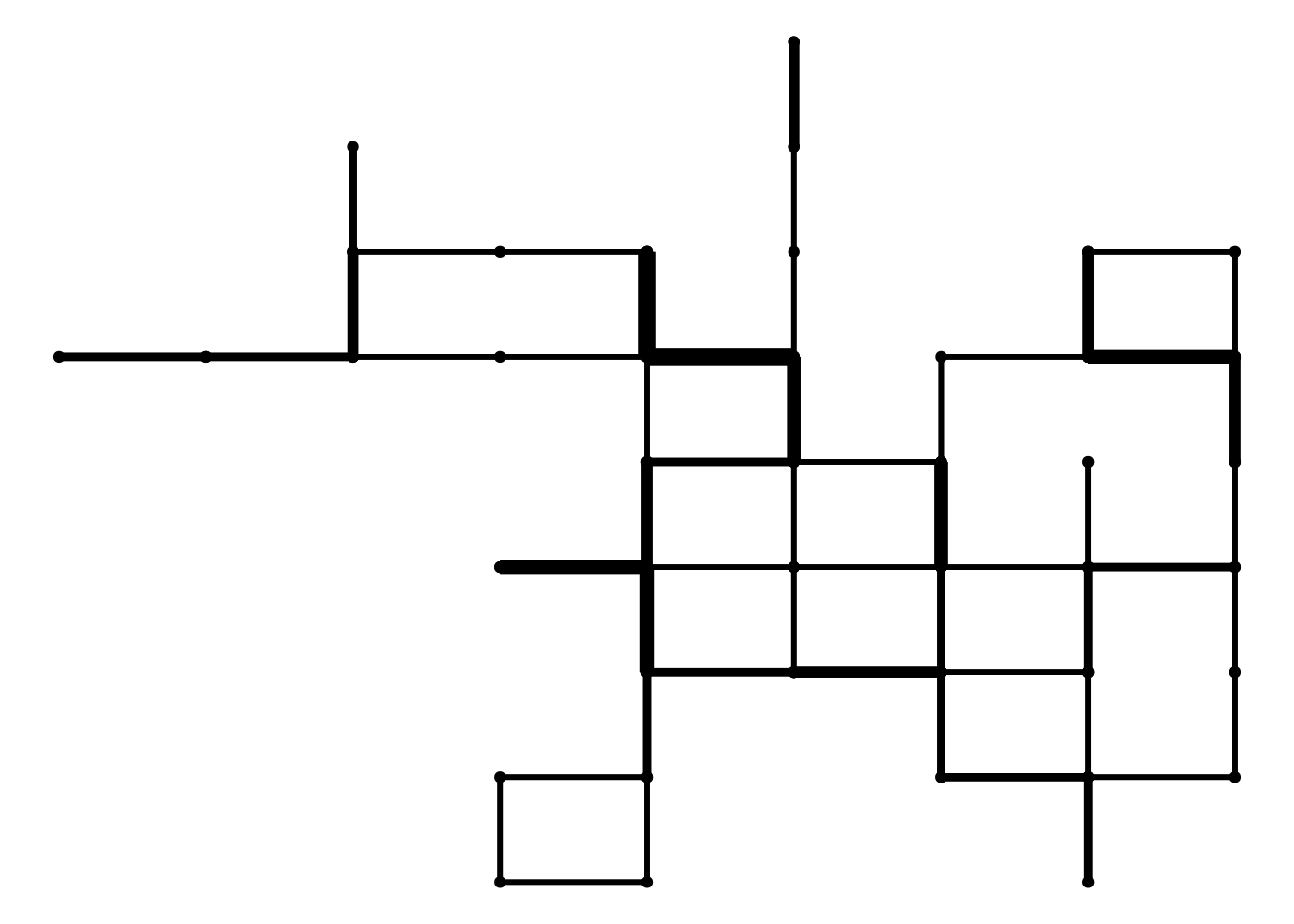

If we set more steps to the random walk, it will cover a much larger area:

set.seed(2222)
rw_1000 <- random_walk(steps = 1000)
plot_random_walk(rw_1000)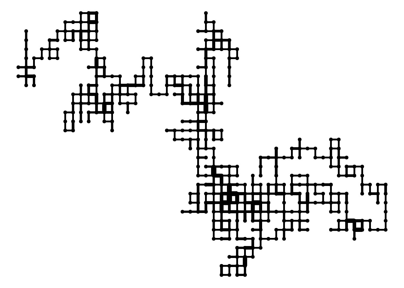

A random walk is a succession of random steps on some mathematical space. We can use random walks to model processes like paths of foraging animals, the evolution of a stock price or the financial status of a gambler. In this post, I have used the functionalities of the tidyverse to generate random walks of lattices of arbitrary number of dimensions, and to plot random walk in two-dimensional lattices.

## R version 4.3.2 (2023-10-31)
## Platform: x86_64-pc-linux-gnu (64-bit)
## Running under: Linux Mint 21.1
## 
## Matrix products: default
## BLAS:   /usr/lib/x86_64-linux-gnu/blas/libblas.so.3.10.0 
## LAPACK: /usr/lib/x86_64-linux-gnu/lapack/liblapack.so.3.10.0
## 
## locale:
##  [1] LC_CTYPE=es_ES.UTF-8       LC_NUMERIC=C              
##  [3] LC_TIME=es_ES.UTF-8        LC_COLLATE=es_ES.UTF-8    
##  [5] LC_MONETARY=es_ES.UTF-8    LC_MESSAGES=es_ES.UTF-8   
##  [7] LC_PAPER=es_ES.UTF-8       LC_NAME=C                 
##  [9] LC_ADDRESS=C               LC_TELEPHONE=C            
## [11] LC_MEASUREMENT=es_ES.UTF-8 LC_IDENTIFICATION=C       
## 
## time zone: Europe/Madrid
## tzcode source: system (glibc)
## 
## attached base packages:
## [1] stats     graphics  grDevices utils     datasets  methods   base     
## 
## other attached packages:
##  [1] lubridate_1.9.2 forcats_1.0.0   stringr_1.5.0   dplyr_1.1.2    
##  [5] purrr_1.0.1     readr_2.1.4     tidyr_1.3.0     tibble_3.2.1   
##  [9] ggplot2_3.4.2   tidyverse_2.0.0
## 
## loaded via a namespace (and not attached):
##  [1] gtable_0.3.3     jsonlite_1.8.4   highr_0.10       compiler_4.3.2  
##  [5] tidyselect_1.2.0 jquerylib_0.1.4  scales_1.2.1     yaml_2.3.7      
##  [9] fastmap_1.1.1    R6_2.5.1         labeling_0.4.2   generics_0.1.3  
## [13] knitr_1.42       bookdown_0.33    munsell_0.5.0    tzdb_0.3.0      
## [17] bslib_0.5.0      pillar_1.9.0     rlang_1.1.0      utf8_1.2.3      
## [21] stringi_1.7.12   cachem_1.0.7     xfun_0.39        sass_0.4.5      
## [25] timechange_0.2.0 cli_3.6.1        withr_2.5.0      magrittr_2.0.3  
## [29] digest_0.6.31    grid_4.3.2       rstudioapi_0.14  hms_1.1.3       
## [33] lifecycle_1.0.3  vctrs_0.6.2      evaluate_0.20    glue_1.6.2      
## [37] farver_2.1.1     blogdown_1.16    fansi_1.0.4      colorspace_2.1-0
## [41] rmarkdown_2.21   tools_4.3.2      pkgconfig_2.0.3  htmltools_0.5.5