The location of facilities is a typical strategic decision in supply chain design. When the potential location of facilities and the potential sources of demand are discrete sets we can define discrete facility location problems.
Facility location problems can have many variants. In the variant I am interested in, we have \(m\) potential facility locations that serve \(n\) demand points. Each potential location has an opening costs \(f_i\), and a maximum capacity \(c_i\). Each demand point requires \(d_j\) units of items. The cost of serving one item from a potential location \(i\) to a demand point \(j\) is proportional to distance \(d_{ij}\).
The formulation of this problem requires the following variables:
- A set of binaries \(y_i\) equal to one if we place a facility in location \(i\) and zero otherwise.
- A set of continuous variables \(x_{ij}\) equal to the demand of \(j\) covered from a facility located at \(i\).
In this post, I intend to solve this problem for the set of capitals of province in peninsular Spain, considering as potential facility locations the ten largest Spanish capitals of provinces, excluding Barcelona and Madrid. This exercise can be seen as an example of prescriptive analytics, as I am trying to find the locations with more potential as logistic centres for this set.
I will be using the tidyverse packages, together with sf and mapSpain for geographical data, and the ompr set of packages to solve linear programming with GLPK. The data of Spanish provincial capitals is stored in the BAdatasetsSpatial package.
library(tidyverse)
library(sf)
library(mapSpain)

library(ompr)
library(ompr.roi)
library(ROI.plugin.glpk)

library(BAdatasetsSpatial)
Distances between Locations
Let’s start finding the values of the parameters with the distances between locations. The latitude, longitude and population of each capital of province is listed in the cap_provincia_es table.
data("cap_provincia_es.rd")## Warning in data("cap_provincia_es.rd"): data set 'cap_provincia_es.rd' not
## foundcap_provincia_es## # A tibble: 52 × 9
## comunidad provincia poblacion latitud longitud altitud habitantes hombres
## <chr> <chr> <chr> <dbl> <dbl> <dbl> <dbl> <dbl>
## 1 Castilla La … Albacete Albacete 39.0 -1.86 686. 169716 83838
## 2 Valencia Alicante… Alicante… 38.3 -0.481 16.6 334757 162853
## 3 Andalucía Almería Almería 36.8 -2.47 27.0 188810 92396
## 4 Extremadura Badajoz Badajoz 38.9 -6.97 192. 148334 72085
## 5 Catalunya Barcelona Barcelona 41.4 2.17 20.0 1621537 771570
## 6 País Vasco Vizcaya Bilbao 43.3 -2.92 17.9 354860 168019
## 7 Castilla León Burgos Burgos 42.3 -3.70 866. 178966 86417
## 8 Valencia Castelló… Castelló… 40.0 -0.0377 36 180005 88979
## 9 Ceuta y Meli… Ceuta Ceuta 35.9 -5.32 13.5 78674 40118
## 10 Castilla La … Ciudad R… Ciudad R… 39.0 -3.93 637. 74014 35073
## # ℹ 42 more rows
## # ℹ 1 more variable: mujeres <dbl>I use the sf::st_as_sf() to set the locations as geographical objects, and then filter the non-peninsular cities. The result is in cap_peninsula_sf.
cap_provincia_es_sf <- st_as_sf(cap_provincia_es,
                               coords = c("longitud", "latitud"),
                               crs = 4326,
                               remove = FALSE)

cap_peninsula_sf <- cap_provincia_es_sf |>
  filter(!comunidad %in% c("Ceuta y Melilla", "Islas Baleares", "Canarias"))
I will calculate the distances between cities with the sf::st_distance() function. Distances are obtained in meters, so I will rescale them as kilometers. The resulting distance matrix is stored in dist_peninsula.
dist_peninsula <- st_distance(cap_peninsula_sf) |>
  units::drop_units()

dist_peninsula <- dist_peninsula / 1000

colnames(dist_peninsula) <- cap_peninsula_sf$poblacion
rownames(dist_peninsula) <- cap_peninsula_sf$poblacion
Defining Potential Facility Locations
The demand points are all the capitals of province in Spain. The demand \(d_j\) is proportional to each citie’s population. It is stored in the demand vector. Here I am also obtaining the number of demand points n.
demand <- cap_peninsula_sf$habitantes
demand <- demand/1000

n <- length(demand)
I need to select the ten most populated areas as potential locations for facilities, excluding Barcelona and Madrid. The positions of these locations in the cap_peninsula_sf table, and therefore in the dist_peninsula matrix, can be obtained with the order() function. Once obtained these positions, I can define the costs matrix of distances from potential locations to demand points.
m <- 10
pos_origins <- order(demand, decreasing = TRUE)[3:(m+2)]
costs <- dist_peninsula[pos_origins, ]
The cities selected as potential locations are:
colnames(dist_peninsula)[pos_origins]## [1] "Valencia" "Sevilla" "Zaragoza" "Málaga"
## [5] "Murcia" "Bilbao" "Alicante/Alacant" "Córdoba"
## [9] "Valladolid" "Coruña (A)"Finally, I am defining the capacity of each of the potential locations capacity and the cost of opening a location open_cost.
capacity <- round(sum(demand)/4) + 100
open_cost <- 3e+05
Building and Solving the Model
Now we are ready to solve the linear programming model. In facility_model I am storing the solution of the model, after parsing it with the ompr syntax.
facility_model <- MIPModel() |>
  add_variable(x[i, j], i = 1:m, j = 1:n, type = "continuous", lb = 0) |>
  add_variable(y[i], i = 1:m, type = "binary", lb = 0) |>
  set_objective(sum_over(costs[i, j]*x[i, j], i = 1:m, j = 1:n) + sum_over(open_cost*y[i], i = 1:m), sense = "min") |>
  add_constraint(sum_over(x[i, j], j = 1:n) <= capacity*y[i], i = 1:m) |>
  add_constraint(sum_over(x[i, j], i = 1:m) >= demand[j], j = 1:n) |>
  solve_model(with_ROI(solver = "glpk"))
Solution
Once solved the model, we can obtain the selected facility locations, which are the ones with \(y_i = 1\).
fac_table <- facility_model |>
  get_solution(y[i]) |>
  mutate(city = rownames(costs)) |>
  filter(value == 1) |>
  relocate(city)
The value of flows from facilities to locations is listed in the \(x_{ij}\) which are nonzero.
facility_model |>
  get_solution(x[i, j]) |>
  mutate(ori = rep(rownames(costs), n),
         des = rep(colnames(costs), each = m)) |>
  filter(value != 0) |>
  relocate(ori, des) |>
  arrange(ori)
## ori des variable i j value
## 1 Bilbao Bilbao x 6 6 354.860
## 2 Bilbao Burgos x 6 7 178.966
## 3 Bilbao Coruña (A) x 6 10 246.056
## 4 Bilbao Donostia-San Sebastián x 6 15 185.357
## 5 Bilbao León x 6 22 134.305
## 6 Bilbao Logroño x 6 24 152.107
## 7 Bilbao Lugo x 6 25 96.678
## 8 Bilbao Oviedo x 6 30 224.005
## 9 Bilbao Pamplona/Iruña x 6 32 198.491
## 10 Bilbao Santander x 6 35 182.700
## 11 Bilbao Vitoria-Gasteiz x 6 44 235.661
## 12 Sevilla Almería x 2 3 188.810
## 13 Sevilla Badajoz x 2 4 148.334
## 14 Sevilla Ciudad Real x 2 9 74.014
## 15 Sevilla Cáceres x 2 12 93.131
## 16 Sevilla Cádiz x 2 13 126.766
## 17 Sevilla Córdoba x 2 14 328.428
## 18 Sevilla Granada x 2 17 234.325
## 19 Sevilla Huelva x 2 19 148.806
## 20 Sevilla Jaén x 2 21 116.557
## 21 Sevilla Málaga x 2 28 568.305
## 22 Sevilla Sevilla x 2 37 703.206
## 23 Valencia Albacete x 1 1 169.716
## 24 Valencia Alicante/Alacant x 1 2 334.757
## 25 Valencia Castellón de la Plana/Castelló de la Plana x 1 8 180.005
## 26 Valencia Cuenca x 1 11 55.866
## 27 Valencia Murcia x 1 27 436.870
## 28 Valencia Teruel x 1 40 35.396
## 29 Valencia Toledo x 1 41 82.291
## 30 Valencia Valencia x 1 42 814.208
## 31 Valladolid Madrid x 9 26 2687.740
## 32 Valladolid Ourense x 9 29 107.742
## 33 Valladolid Palencia x 9 31 82.651
## 34 Valladolid Pontevedra x 9 33 81.576
## 35 Valladolid Salamanca x 9 34 155.619
## 36 Valladolid Segovia x 9 36 56.660
## 37 Valladolid Valladolid x 9 43 317.864
## 38 Valladolid Zamora x 9 45 66.293
## 39 Valladolid Ávila x 9 47 56.855
## 40 Zaragoza Barcelona x 3 5 1621.537
## 41 Zaragoza Girona x 3 16 96.188
## 42 Zaragoza Guadalajara x 3 18 83.039
## 43 Zaragoza Huesca x 3 20 52.059
## 44 Zaragoza Lleida x 3 23 135.919
## 45 Zaragoza Madrid x 3 26 568.204
## 46 Zaragoza Soria x 3 38 39.528
## 47 Zaragoza Tarragona x 3 39 140.323
## 48 Zaragoza Zaragoza x 3 46 674.317Plotting the Solution
Now I will use the mapSpain package to plot the flows from facilities to demand points. To distinguish facilities from demand points, I create the facility column in the cap_peninsula_sf table.
facilities <- fac_table$city

cap_peninsula_sf <- cap_peninsula_sf |>
  mutate(pos = 1:n(),
         facility = ifelse(poblacion %in% facilities, "fac", "not_fac"))
To represent flows, I need to plot lines as spatial objects. First, I am picking the list of edges from the model solution, excluding the flows with origin and destination in the same city. The result is stored in the edges data fram.e
edges <- facility_model |>
  get_solution(x[i, j]) |>
  mutate(ori = rep(rownames(costs), n),
         des = rep(colnames(costs), each = m)) |>
  filter(value != 0, ori != des) |>
  select(i, j)
Then, I need to get the latitude and longitude of the origin and destination of each edge. To avoid uncontrolled column renaming, I obtain two tables of coordinates with renamed longitude and latitude columns.
ori_coord <- cap_peninsula_sf |>
  st_drop_geometry() |>
  slice(pos_origins) |>
  select(longitud, latitud) |>
  mutate(i = 1:n()) |>
  rename(lon_x = longitud, lat_x = latitud)

des_coord <- cap_peninsula_sf |>
  st_drop_geometry() |>
  select(longitud, latitud) |>
  mutate(j = 1:n()) |>
  rename(lon_y = longitud, lat_y = latitud)
Then, I can add safely origin and destination coordinates to the edges list.
edges <- edges |>
  left_join(ori_coord, by = "i") |>
  left_join(des_coord, by = "j")
As I need a geometry column of line objects, I need to obtain these lines as a list of spatial objectes with purrr:pmap() and sf::st_linestring().
lines <- pmap(edges,
              ~ st_linestring(matrix(c(..3, ..4, ..5, ..6),
                                     2, 2, byrow = TRUE)))
Then, I use sf::st_sfc() and sf::st_sf() to obtain a geometry column of lines. The result is stored in the edges_sf table.
edges_sf <- st_sf(edges,
                  geometry = st_sfc(lines, crs = 4326))
edges_sf
## Simple feature collection with 43 features and 6 fields
## Geometry type: LINESTRING
## Dimension: XY
## Bounding box: xmin: -8.648053 ymin: 36.52969 xmax: 2.8237 ymax: 43.46096
## Geodetic CRS: WGS 84
## First 10 features:
## i j lon_x lat_x lon_y lat_y geometry
## 1 1 1 -0.3768049 39.47024 -1.8600700 38.99765 LINESTRING (-0.3768049 39.4...
## 2 1 2 -0.3768049 39.47024 -0.4810060 38.34520 LINESTRING (-0.3768049 39.4...
## 3 2 3 -5.9962950 37.38264 -2.4679220 36.84016 LINESTRING (-5.996295 37.38...
## 4 2 4 -5.9962950 37.38264 -6.9702840 38.87860 LINESTRING (-5.996295 37.38...
## 5 3 5 -0.8765379 41.65629 2.1699190 41.38792 LINESTRING (-0.8765379 41.6...
## 6 6 7 -2.9234410 43.25696 -3.6997310 42.34087 LINESTRING (-2.923441 43.25...
## 7 1 8 -0.3768049 39.47024 -0.0376709 39.98598 LINESTRING (-0.3768049 39.4...
## 8 2 9 -5.9962950 37.38264 -3.9272630 38.98610 LINESTRING (-5.996295 37.38...
## 9 6 10 -2.9234410 43.25696 -8.3958350 43.37087 LINESTRING (-2.923441 43.25...
## 10 1 11 -0.3768049 39.47024 -2.1340050 40.07183 LINESTRING (-0.3768049 39.4...Now that I have the points stored at cap_peninsula_sf and the lines at edges_sf, I can do the plot with the mapSpain::esp_get_prov_siane() map.
esp_get_prov_siane(epsg = "4326") |>
  ggplot() +
  geom_sf(fill = "white") +
  geom_sf(data = cap_peninsula_sf, aes(color = facility)) +
  geom_sf(data = edges_sf) +
  theme_void() +
  theme(legend.position = "none")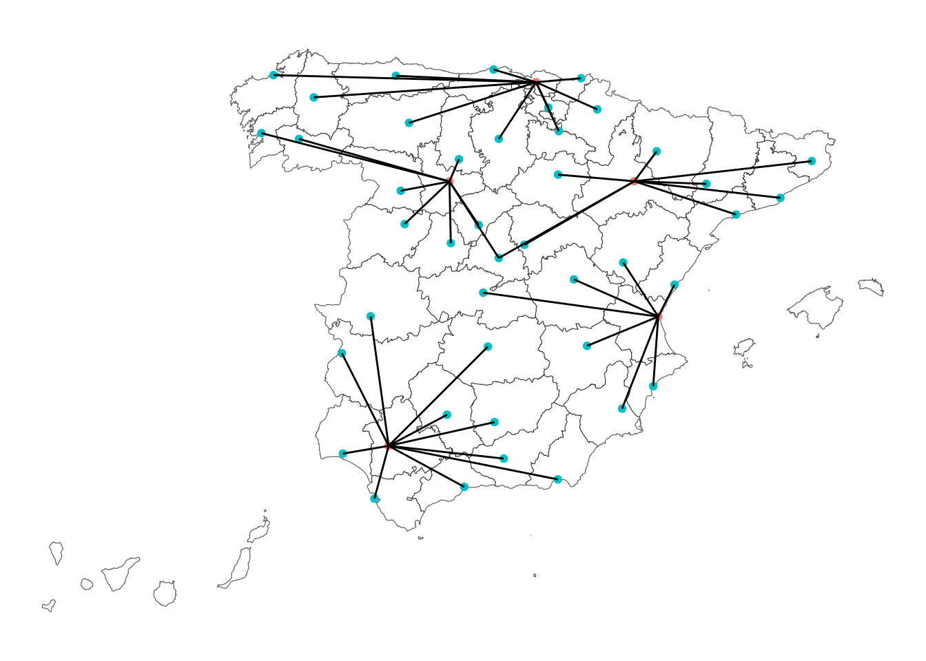
The map shows the relevance of largely populated capitals of coastal provinces like Bilbao, Sevilla and Valencia. Valladolid covers part of de demand of Madrid and Castilian and Galician cities. Finally, Zaragoza takes advantage of its position between Barcelona and Madrid. A more accurate assessment of the potential of facility locations could be obtained using the list of all Spanish towns and cities, which can be obtained at BAdatasetsSpatial::poblaciones_es.
References
mapSpainpackage: https://github.com/rOpenSpain/mapSpain, https://rpubs.com/dieghernan/mapSpain_mapas_Romprpackage: https://dirkschumacher.github.io/ompr/
Session Info
sessionInfo()## R version 4.5.3 (2026-03-11)
## Platform: x86_64-pc-linux-gnu
## Running under: Linux Mint 21.1
##
## Matrix products: default
## BLAS: /usr/lib/x86_64-linux-gnu/blas/libblas.so.3.10.0
## LAPACK: /usr/lib/x86_64-linux-gnu/lapack/liblapack.so.3.10.0 LAPACK version 3.10.0
##
## locale:
## [1] LC_CTYPE=es_ES.UTF-8 LC_NUMERIC=C
## [3] LC_TIME=es_ES.UTF-8 LC_COLLATE=es_ES.UTF-8
## [5] LC_MONETARY=es_ES.UTF-8 LC_MESSAGES=es_ES.UTF-8
## [7] LC_PAPER=es_ES.UTF-8 LC_NAME=C
## [9] LC_ADDRESS=C LC_TELEPHONE=C
## [11] LC_MEASUREMENT=es_ES.UTF-8 LC_IDENTIFICATION=C
##
## time zone: Europe/Madrid
## tzcode source: system (glibc)
##
## attached base packages:
## [1] stats graphics grDevices utils datasets methods base
##
## other attached packages:
## [1] BAdatasetsSpatial_0.1.0 ROI.plugin.glpk_1.0-0 ompr.roi_1.0.2
## [4] ompr_1.0.4 mapSpain_0.10.0 sf_1.0-20
## [7] lubridate_1.9.4 forcats_1.0.1 stringr_1.6.0
## [10] dplyr_1.1.4 purrr_1.2.0 readr_2.1.5
## [13] tidyr_1.3.1 tibble_3.3.0 ggplot2_4.0.0
## [16] tidyverse_2.0.0
##
## loaded via a namespace (and not attached):
## [1] gtable_0.3.6 xfun_0.52 bslib_0.9.0
## [4] lattice_0.22-9 numDeriv_2016.8-1.1 tzdb_0.5.0
## [7] vctrs_0.6.5 tools_4.5.3 generics_0.1.3
## [10] proxy_0.4-27 pkgconfig_2.0.3 Matrix_1.7-4
## [13] KernSmooth_2.23-26 data.table_1.17.8 checkmate_2.3.2
## [16] RColorBrewer_1.1-3 S7_0.2.0 listcomp_0.4.1
## [19] lifecycle_1.0.4 compiler_4.5.3 farver_2.1.2
## [22] htmltools_0.5.8.1 class_7.3-23 sass_0.4.10
## [25] yaml_2.3.10 lazyeval_0.2.2 pillar_1.11.1
## [28] jquerylib_0.1.4 classInt_0.4-11 cachem_1.1.0
## [31] wk_0.9.4 tidyselect_1.2.1 digest_0.6.37
## [34] slam_0.1-50 stringi_1.8.7 bookdown_0.43
## [37] fastmap_1.2.0 grid_4.5.3 cli_3.6.4
## [40] magrittr_2.0.4 utf8_1.2.4 e1071_1.7-16
## [43] withr_3.0.2 rappdirs_0.3.3 scales_1.4.0
## [46] backports_1.5.0 registry_0.5-1 timechange_0.3.0
## [49] rmarkdown_2.29 blogdown_1.21 hms_1.1.4
## [52] ROI_1.0-1 evaluate_1.0.3 knitr_1.50
## [55] Rglpk_0.6-5.1 s2_1.1.7 rlang_1.1.6
## [58] Rcpp_1.1.0 glue_1.8.0 DBI_1.2.3
## [61] rstudioapi_0.17.1 jsonlite_2.0.0 R6_2.6.1
## [64] units_0.8-7