The ggplot2 package is a system to create graphics in the context of the tidyverse, using the grammar of graphics. The elements of a ggplot are:

• A dataset, usually passed as a data frame. We obtain the best from ggplot if the data frame is in tidy format.
• A mapping, defined as a set of instructions on how parts of the data are mapped onto aesthetic attributes of geometric objects. The mapping is passed using the aes() function. Here we establish which variables will be used in the plot axis, and which variables will be used for coloring or shaping plot elements.
• A set of layers, which define how the data will be displayed in the plot. They include the geometric element or geom (points, lines, bars, etc.) and the statistical transformation or stats required to make the plot.

In this post, I will shortly introduce how to control aesthetic evaluation in ggplot, mostly using the afer_stat() function in the mapping of the plot. To do so, we need to load the tidyverse to access ggplot2:

library(tidyverse)

We can see an example of the default use of stats with this simple plot:

ggplot(mpg, aes(class)) +
  geom_bar()

Let’s examine the elements of this plot:

• The dataset mpg, which is loaded with ggplot2.
• The mapping of the plot consists of setting the class factor variable in the x axis (the first two arguments of aes() are the variables of the data frame to be set in the x and y axis).
• We define a bar plot with geom_bar().

To do this plot, ggplot2 has counted how many rows of the dataset belong to each level, stored the result of the count variable and mapped this variable in the y axis. count is an example of a stat, a variable generated internally by ggplot. In fact, a layer in ggplot consists of two elements: the statistical transformations or stats, and the geometry geoms. The stat performs the computations required to build the graphic, and the geom part controls how the plot is displayed.

We use after_stat() to transform the y axis establishing the relative frequency of each level. This proportion is calculated as count/sum(count).

ggplot(mpg, aes(x = class, y = after_stat(count / sum(count)))) +
  geom_bar()

To appreciate the difference between the two plots, examine the values of the y axis. In the first plot they are the total count, in the second the proportion of each variable.

To see which variables are computed in a geom_*(), check the Computed variables section of the reference page or help. For instance, for the histograms we have:

• the count of observations of each bin.
• the density of points in bin, scaled to integrate to 1.
• the variables ncount and ndensity, scaled to a maximum of 1.

The default stat for histograms is count (see label of y axis):

ggplot(mpg, aes(hwy)) +
  geom_histogram(bins = 20)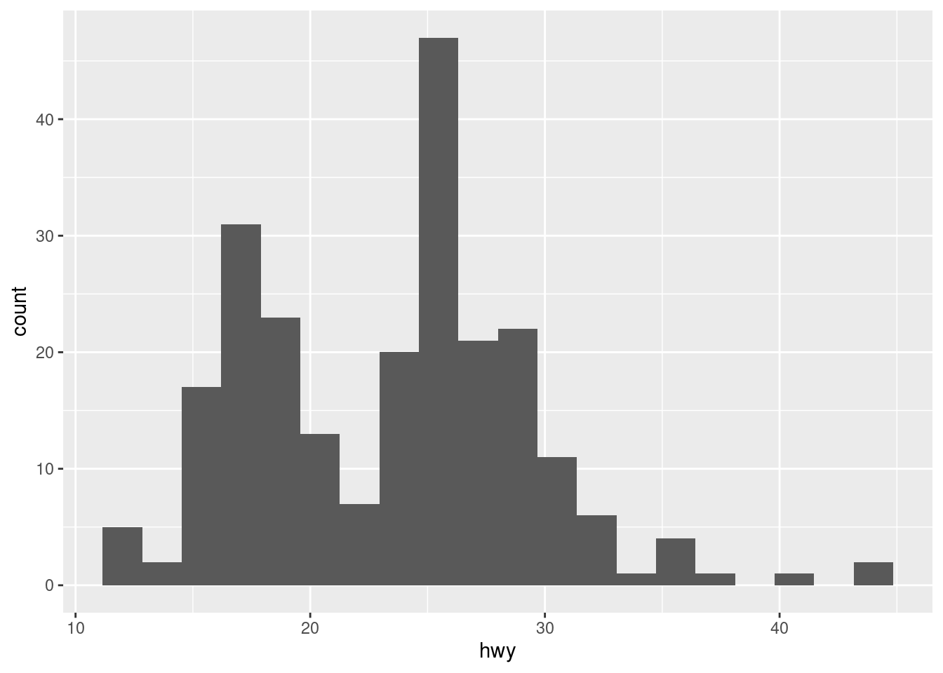

Here is the relative frequency, scaled so that the sum of heights of bars is equal to one:

ggplot(mpg, aes(hwy, y = after_stat(count / sum(count)))) +
  geom_histogram(bins = 20)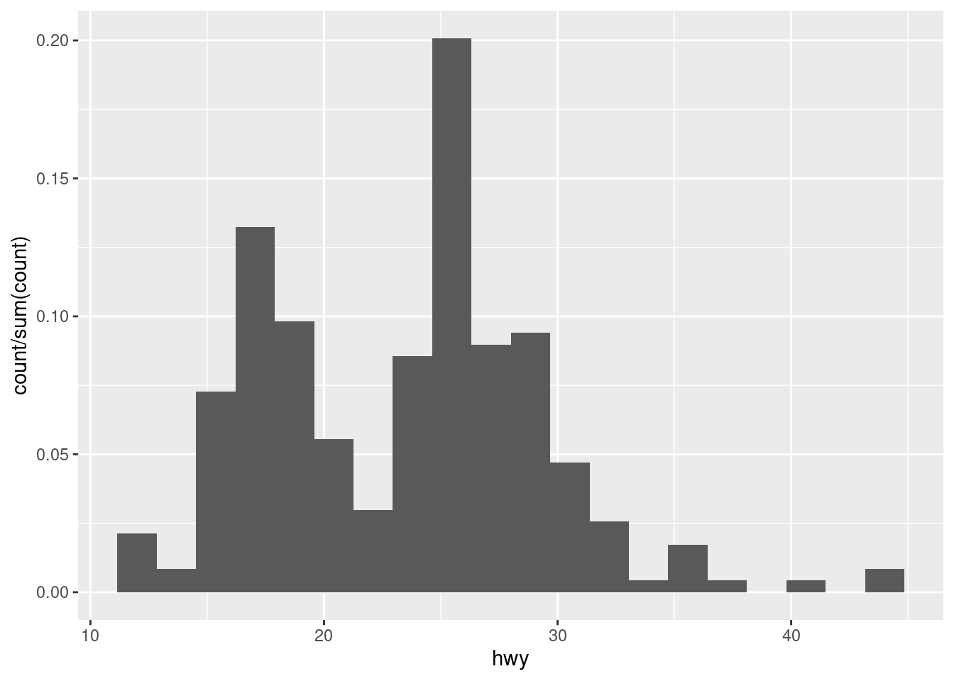

Below is the result of using density. The heigth of bars is scaled so that the total area of bins is equal to 1. The line obtained with geom_density() is computed tending the number of bins to infinity. This scaling allows the two geoms being superimposed.

ggplot(mpg, aes(hwy, y = after_stat(density))) +
  geom_histogram(bins = 20, fill = "#A0A0A0") +
  geom_density(linewidth = 2)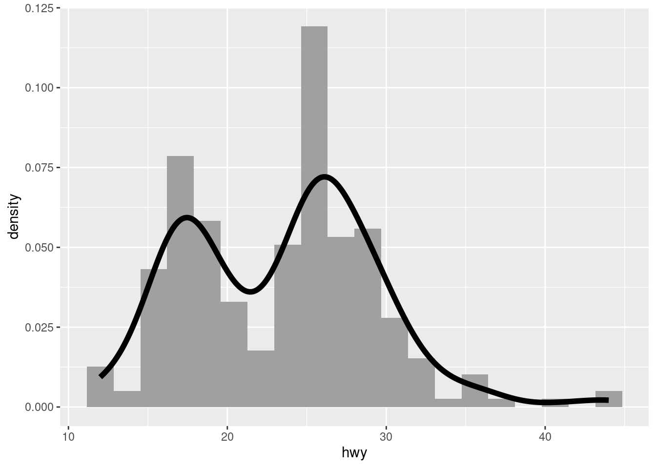

Each geom_*() has a stat variable, indicating which stat to use when calculating layer parameters. The most frequent default is stat = "identity", but it can be useful to pass a different parameter. Let’s see how can we set the value of counts in a barplot.

ggplot(mpg, aes(class)) +
  geom_bar() +
  geom_text(aes(y = after_stat(count + 2), label = after_stat(count)), 
            stat = "count")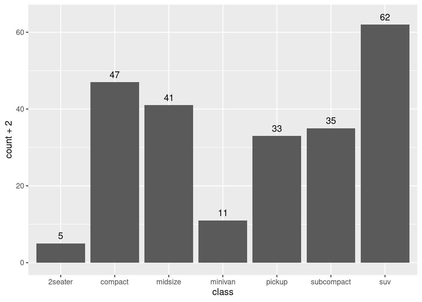

The aes() function of geom_text() has three parameters:

• The x axis, inherited from the aesthetics of ggplot().
• The y axis, equal to the count of each bar plus two.
• The label, equal to the actual count.

To be able to calculate the counts, we need to set stat = "count" for geom_text().

Let’s see another example of use of stats with boxplots.

ggplot(iris, aes(Species, Sepal.Length)) +
  geom_boxplot() +
  geom_text(aes(y = stage(Sepal.Length, after_stat = ymax), 
                label = after_stat(paste(ymax, "-", ymin))), 
                stat = "boxplot", vjust = - 0.5)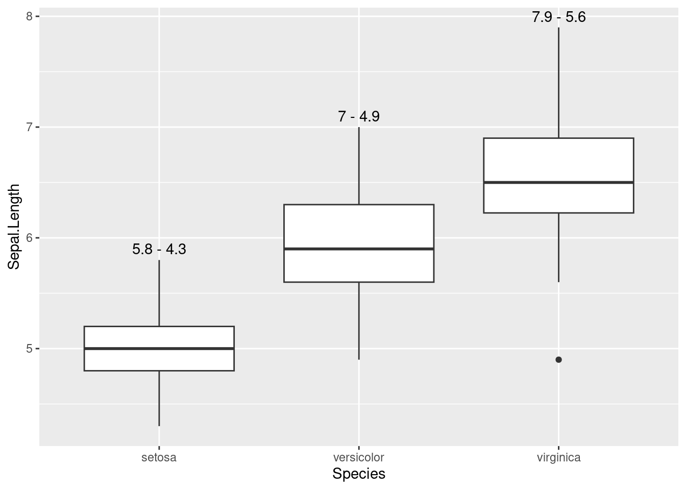

In the first two lines of the plot, I am making a boxplot for each value of Species. Then, I am placing a label with geom_text() as follows:

• I want to position the label in the ymax value of the boxplot. That’s why I am setting stat = "boxplot" for this geom.
• The y axis is the ymax variable of geom_boxplot(). To obtain it, I need to use stage() to pass the Sepal.Length variable.
• the label is an expression from ymax and ymin.

A layer in ggplot consists of two elements: the statistical transformations or stats, and the geometry geoms. The stat performs the computations required to build the graphic, and the geom part controls how the plot is displayed. The variables calculated in the stat can be checked in the Computed variables section of the geom reference. We can use functions such as after_stat() or stage() to use these computed variables in our plots.

## R version 4.5.1 (2025-06-13)
## Platform: x86_64-pc-linux-gnu
## Running under: Linux Mint 21.1
## 
## Matrix products: default
## BLAS:   /usr/lib/x86_64-linux-gnu/blas/libblas.so.3.10.0 
## LAPACK: /usr/lib/x86_64-linux-gnu/lapack/liblapack.so.3.10.0  LAPACK version 3.10.0
## 
## locale:
##  [1] LC_CTYPE=es_ES.UTF-8       LC_NUMERIC=C              
##  [3] LC_TIME=es_ES.UTF-8        LC_COLLATE=es_ES.UTF-8    
##  [5] LC_MONETARY=es_ES.UTF-8    LC_MESSAGES=es_ES.UTF-8   
##  [7] LC_PAPER=es_ES.UTF-8       LC_NAME=C                 
##  [9] LC_ADDRESS=C               LC_TELEPHONE=C            
## [11] LC_MEASUREMENT=es_ES.UTF-8 LC_IDENTIFICATION=C       
## 
## time zone: Europe/Madrid
## tzcode source: system (glibc)
## 
## attached base packages:
## [1] stats     graphics  grDevices utils     datasets  methods   base     
## 
## other attached packages:
##  [1] lubridate_1.9.4 forcats_1.0.0   stringr_1.5.2   dplyr_1.1.4    
##  [5] purrr_1.1.0     readr_2.1.5     tidyr_1.3.1     tibble_3.3.0   
##  [9] ggplot2_4.0.0   tidyverse_2.0.0
## 
## loaded via a namespace (and not attached):
##  [1] gtable_0.3.6       jsonlite_2.0.0     compiler_4.5.1     tidyselect_1.2.1  
##  [5] jquerylib_0.1.4    scales_1.4.0       yaml_2.3.10        fastmap_1.2.0     
##  [9] R6_2.6.1           labeling_0.4.3     generics_0.1.3     knitr_1.50        
## [13] bookdown_0.43      tzdb_0.5.0         bslib_0.9.0        pillar_1.11.1     
## [17] RColorBrewer_1.1-3 rlang_1.1.6        stringi_1.8.7      cachem_1.1.0      
## [21] xfun_0.52          sass_0.4.10        S7_0.2.0           timechange_0.3.0  
## [25] cli_3.6.4          withr_3.0.2        magrittr_2.0.4     digest_0.6.37     
## [29] grid_4.5.1         rstudioapi_0.17.1  hms_1.1.3          lifecycle_1.0.4   
## [33] vctrs_0.6.5        evaluate_1.0.3     glue_1.8.0         farver_2.1.2      
## [37] blogdown_1.21      rmarkdown_2.29     tools_4.5.1        pkgconfig_2.0.3   
## [41] htmltools_0.5.8.1