In this post, I will present how to plot a faceted bar plot. The challenge in defining such a graph is that the ordering of elements across facets can change. To allow this, we need the reorder_within() and “scale_y_reordered()` from the tidytext package.
As an example, I will present the countries with the lowest fertility rates across different years. I will retrieve the World Bank data with the wbstats package and add additional information with the countrycode package.
library(wbstats)
library(countrycode)
library(tidyverse)
library(tidytext)
I start retrieving total fertility rate with the wbstats::wb_data() function.
tfrt_data <- wb_data("SP.DYN.TFRT.IN", start_date = 2000, end_date = 2022) |>
  select(iso2c:SP.DYN.TFRT.IN)
Let’s see the ten countries with lower fertility rates in years 2000, 2015 and 2022. We can do that using the purrr::walk()function.
walk(c(2000, 2015, 2022), ~ {
  tfrt_data |>
  filter(date == .) |>
  arrange(SP.DYN.TFRT.IN) |>
  print(n = 10)
})
## # A tibble: 217 × 5
## iso2c iso3c country date SP.DYN.TFRT.IN
## <chr> <chr> <chr> <dbl> <dbl>
## 1 MO MAC Macao SAR, China 2000 0.912
## 2 HK HKG Hong Kong SAR, China 2000 1.03
## 3 UA UKR Ukraine 2000 1.12
## 4 CZ CZE Czechia 2000 1.15
## 5 RU RUS Russian Federation 2000 1.20
## 6 ES ESP Spain 2000 1.22
## 7 GR GRC Greece 2000 1.25
## 8 LV LVA Latvia 2000 1.25
## 9 BG BGR Bulgaria 2000 1.26
## 10 IT ITA Italy 2000 1.26
## # ℹ 207 more rows
## # A tibble: 217 × 5
## iso2c iso3c country date SP.DYN.TFRT.IN
## <chr> <chr> <chr> <dbl> <dbl>
## 1 VG VGB British Virgin Islands 2015 1.19
## 2 HK HKG Hong Kong SAR, China 2015 1.20
## 3 MO MAC Macao SAR, China 2015 1.20
## 4 KR KOR Korea, Rep. 2015 1.24
## 5 SG SGP Singapore 2015 1.24
## 6 BA BIH Bosnia and Herzegovina 2015 1.29
## 7 PT PRT Portugal 2015 1.31
## 8 PL POL Poland 2015 1.32
## 9 CY CYP Cyprus 2015 1.33
## 10 GR GRC Greece 2015 1.33
## # ℹ 207 more rows
## # A tibble: 217 × 5
## iso2c iso3c country date SP.DYN.TFRT.IN
## <chr> <chr> <chr> <dbl> <dbl>
## 1 HK HKG Hong Kong SAR, China 2022 0.701
## 2 KR KOR Korea, Rep. 2022 0.778
## 3 PR PRI Puerto Rico 2022 0.9
## 4 VG VGB British Virgin Islands 2022 1.01
## 5 SG SGP Singapore 2022 1.04
## 6 MO MAC Macao SAR, China 2022 1.11
## 7 MT MLT Malta 2022 1.15
## 8 ES ESP Spain 2022 1.16
## 9 CN CHN China 2022 1.18
## 10 AW ABW Aruba 2022 1.18
## # ℹ 207 more rowsWe observe that the ranking has been shifting during the three selected years. Let’s retrieve the ten main countries in each year and save them in the tfrt_shortlist table.
tfrt_shortlist <- tfrt_data |>
  filter(date %in% c(2000, 2015, 2022)) |>
  group_by(date) |>
  arrange(SP.DYN.TFRT.IN) |>
  slice(1:10) |>
  ungroup()
It can be interesting to add information about the continent of each country, using the countrycode::countrycode() package.
tfrt_shortlist <- tfrt_shortlist |>
  mutate(continent = countrycode(iso2c, origin = "iso2c", destination = "continent"))
Let’s try to do a vertical chart of fertility rate for each year using a faceted barplot.
tfrt_shortlist |>
  mutate(country = fct_reorder(country, SP.DYN.TFRT.IN)) |>
  ggplot(aes(SP.DYN.TFRT.IN, country, fill = continent)) +
  geom_col() +
  facet_grid(date ~ .)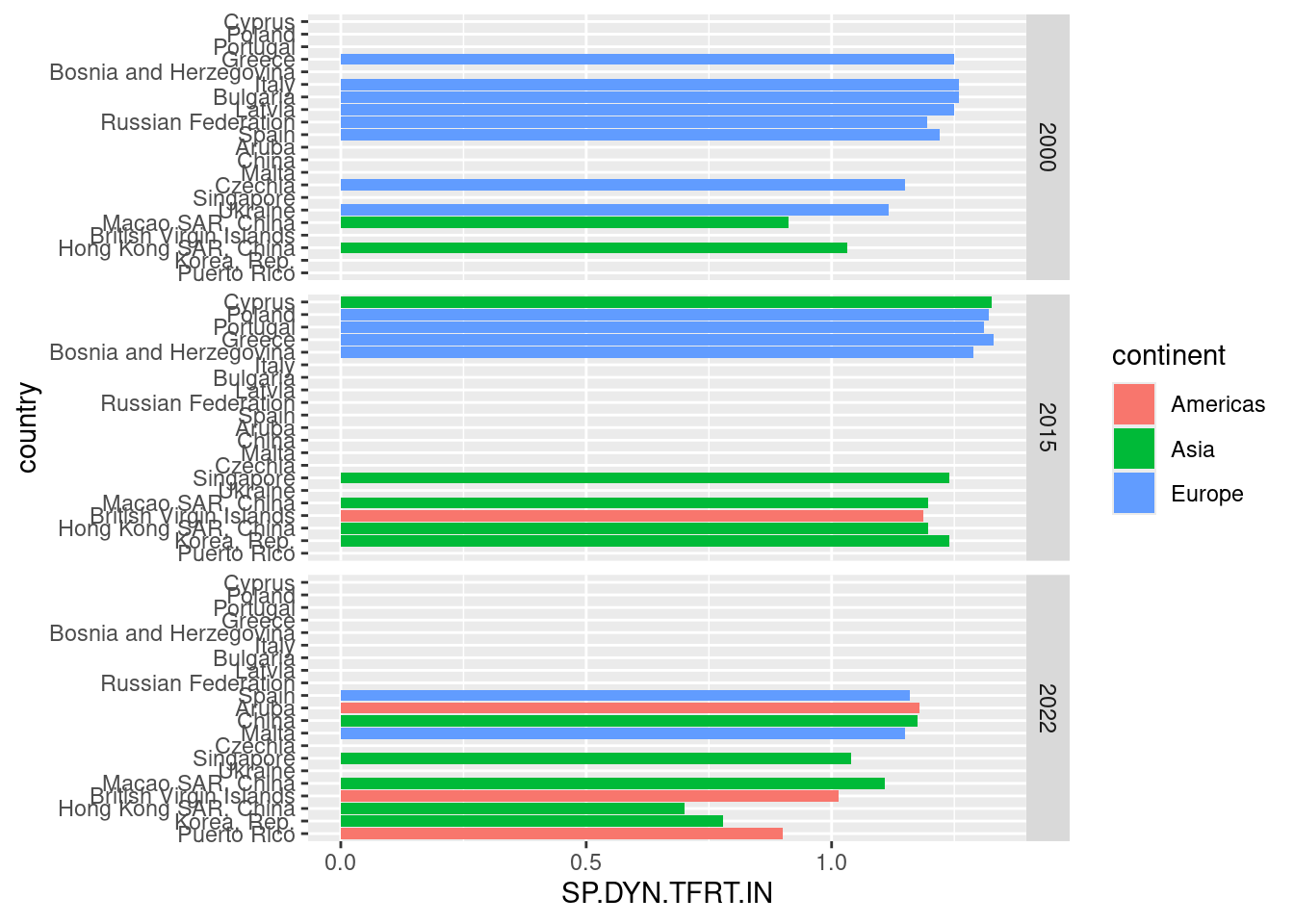
We observe that the plot has several flaws:
- The order of each facet is the same for all years.
- All involved countries appear in each facet, even if they do not appear in the ranking of each year.
To remedy this, we can use the functions reoder_within() and scale_y_reordered() from the tidytext package. The function reorder_within() replaces forcats::fct_reorder().
tfrt_shortlist |>
  mutate(country = reorder_within(country, -SP.DYN.TFRT.IN, date)) |>
  ggplot(aes(SP.DYN.TFRT.IN, country, fill = continent)) +
  geom_col() +
  scale_y_reordered() +
  facet_grid(date ~ ., scales = "free_y")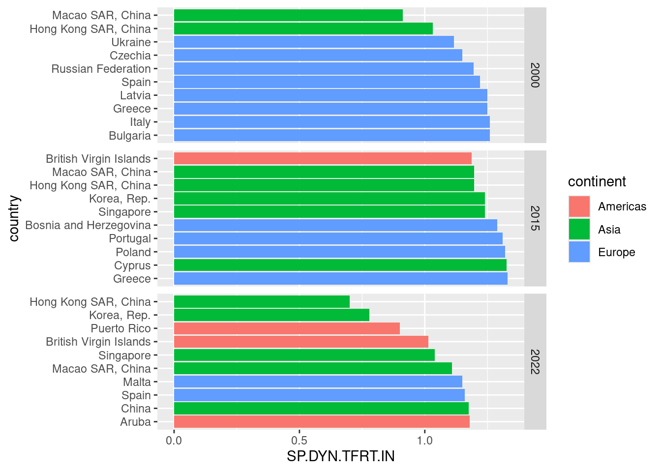
Once achieved the reordering within each facet, we can proceed to present the final plot.
tfrt_shortlist |>
  mutate(country = reorder_within(country, -SP.DYN.TFRT.IN, date)) |>
  ggplot(aes(SP.DYN.TFRT.IN, country, fill = continent)) +
  geom_col() +
  scale_y_reordered() +
  facet_grid(date ~ ., scales = "free_y") +
  labs(title = "Evolution of lowest fertility rates", x = NULL, y = NULL) +
  theme_linedraw(base_size = 10) +
  theme(legend.position = "bottom", plot.title.position = "plot")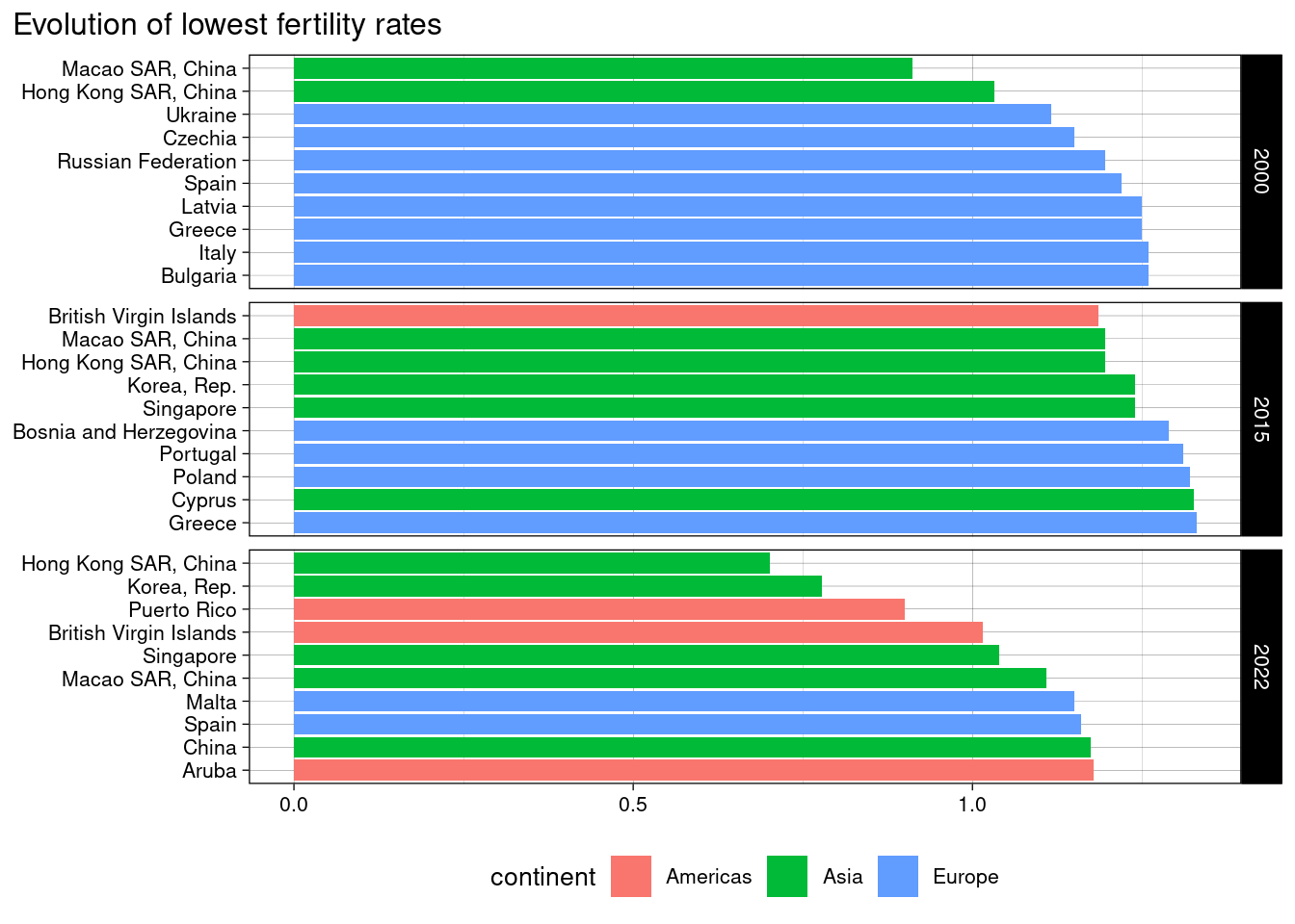
Reference
- World Bank Data. Fertility rate, total (births per woman). https://data.worldbank.org/indicator/SP.DYN.TFRT.IN
Session Info
## R version 4.4.1 (2024-06-14)
## Platform: x86_64-pc-linux-gnu
## Running under: Linux Mint 21.1
##
## Matrix products: default
## BLAS:   /usr/lib/x86_64-linux-gnu/blas/libblas.so.3.10.0
## LAPACK: /usr/lib/x86_64-linux-gnu/lapack/liblapack.so.3.10.0
##
## locale:
##  [1] LC_CTYPE=es_ES.UTF-8       LC_NUMERIC=C
##  [3] LC_TIME=es_ES.UTF-8        LC_COLLATE=es_ES.UTF-8
##  [5] LC_MONETARY=es_ES.UTF-8    LC_MESSAGES=es_ES.UTF-8
##  [7] LC_PAPER=es_ES.UTF-8       LC_NAME=C
##  [9] LC_ADDRESS=C               LC_TELEPHONE=C
## [11] LC_MEASUREMENT=es_ES.UTF-8 LC_IDENTIFICATION=C
##
## time zone: Europe/Madrid
## tzcode source: system (glibc)
##
## attached base packages:
## [1] stats     graphics  grDevices utils     datasets  methods   base
##
## other attached packages:
##  [1] tidytext_0.4.2    lubridate_1.9.3   forcats_1.0.0     stringr_1.5.1
##  [5] dplyr_1.1.4       purrr_1.0.2       readr_2.1.5       tidyr_1.3.1
##  [9] tibble_3.2.1      ggplot2_3.5.1     tidyverse_2.0.0   countrycode_1.6.0
## [13] wbstats_1.0.4
##
## loaded via a namespace (and not attached):
##  [1] janeaustenr_1.0.0 sass_0.4.9        utf8_1.2.4        generics_0.1.3
##  [5] lattice_0.22-5    blogdown_1.19     stringi_1.8.3     hms_1.1.3
##  [9] digest_0.6.35     magrittr_2.0.3    evaluate_0.23     grid_4.4.1
## [13] timechange_0.3.0  bookdown_0.39     fastmap_1.1.1     Matrix_1.6-5
## [17] jsonlite_1.8.8    httr_1.4.7        fansi_1.0.6       scales_1.3.0
## [21] jquerylib_0.1.4   cli_3.6.2         rlang_1.1.3       tokenizers_0.3.0
## [25] munsell_0.5.1     withr_3.0.0       cachem_1.0.8      yaml_2.3.8
## [29] tools_4.4.1       tzdb_0.4.0        colorspace_2.1-0  curl_5.2.1
## [33] vctrs_0.6.5       R6_2.5.1          lifecycle_1.0.4   pkgconfig_2.0.3
## [37] pillar_1.9.0      bslib_0.7.0       gtable_0.3.5      Rcpp_1.0.12
## [41] glue_1.7.0        highr_0.10        xfun_0.43         tidyselect_1.2.1
## [45] rstudioapi_0.16.0 knitr_1.46        farver_2.1.1      SnowballC_0.7.1
## [49] htmltools_0.5.8.1 labeling_0.4.3    rmarkdown_2.26    compiler_4.4.1