In this post, I will present visualizations of financial data presented in the tidytuesday challenge Big Tech Stock Prices. In addition to line plots, I will present how to do a candlestick plot using ggplot. I will be using the geom_segment() and scale_x_date() to do the plots.
In addition to the tidyverse, I will use kableExtra to present tabular data.
library(tidyverse)
library(kableExtra)
You can get the stock prices data from tidytuesday by doing:
tuesdata <- tidytuesdayR::tt_load('2023-02-07')
tuesdata <- tidytuesdayR::tt_load(2023, week = 6)

big_tech_stock_prices <- tuesdata$big_tech_stock_prices
big_tech_companies <- tuesdata$big_tech_companies
The big_tech_companies table contains the stock sign and company name:
big_tech_companies |>
  kbl() |>
kable_styling(full_width = FALSE)| stock_symbol | company |
|---|---|
| AAPL | Apple Inc. |
| ADBE | Adobe Inc. |
| AMZN | Amazon.com, Inc. |
| CRM | Salesforce, Inc. |
| CSCO | Cisco Systems, Inc. |
| GOOGL | Alphabet Inc. |
| IBM | International Business Machines Corporation |
| INTC | Intel Corporation |
| META | Meta Platforms, Inc. |
| MSFT | Microsoft Corporation |
| NFLX | Netflix, Inc. |
| NVDA | NVIDIA Corporation |
| ORCL | Oracle Corporation |
| TSLA | Tesla, Inc. |
In big_tech_stock_prices, for each day stocks are traded, we have:
- The
highand low price of the session. - The
openandcloseprice of the session.adj_closeis an adjusted closing price accounting for applicable splits and dividend distributions. I will be usingadj_closeas value of closing price as it is more representative.
big_tech_stock_prices |>
  slice(1:10) |>
  kbl() |>
kable_styling(full_width = FALSE)| stock_symbol | date | open | high | low | close | adj_close | volume |
|---|---|---|---|---|---|---|---|
| AAPL | 2010-01-04 | 7.622500 | 7.660714 | 7.585000 | 7.643214 | 6.515213 | 493729600 |
| AAPL | 2010-01-05 | 7.664286 | 7.699643 | 7.616071 | 7.656429 | 6.526476 | 601904800 |
| AAPL | 2010-01-06 | 7.656429 | 7.686786 | 7.526786 | 7.534643 | 6.422664 | 552160000 |
| AAPL | 2010-01-07 | 7.562500 | 7.571429 | 7.466071 | 7.520714 | 6.410790 | 477131200 |
| AAPL | 2010-01-08 | 7.510714 | 7.571429 | 7.466429 | 7.570714 | 6.453412 | 447610800 |
| AAPL | 2010-01-11 | 7.600000 | 7.607143 | 7.444643 | 7.503929 | 6.396483 | 462229600 |
| AAPL | 2010-01-12 | 7.471071 | 7.491786 | 7.372143 | 7.418571 | 6.323721 | 594459600 |
| AAPL | 2010-01-13 | 7.423929 | 7.533214 | 7.289286 | 7.523214 | 6.412922 | 605892000 |
| AAPL | 2010-01-14 | 7.503929 | 7.516429 | 7.465000 | 7.479643 | 6.375781 | 432894000 |
| AAPL | 2010-01-15 | 7.533214 | 7.557143 | 7.352500 | 7.354643 | 6.269228 | 594067600 |
Some Line Plots
The dataset allows visualizing how stock prices of big tech companies have risen during the last decades, and collapsed recently.
big_tech_stock_prices |>
  filter(stock_symbol == "AMZN") |>
  ggplot(aes(date, adj_close)) +
  geom_line(color = "#606060") +
  theme_minimal() +
  scale_x_date(name = NULL, date_breaks = "1 year", date_labels = "%Y") +
  labs(title = "Evolution of AMZN price stock", y = NULL)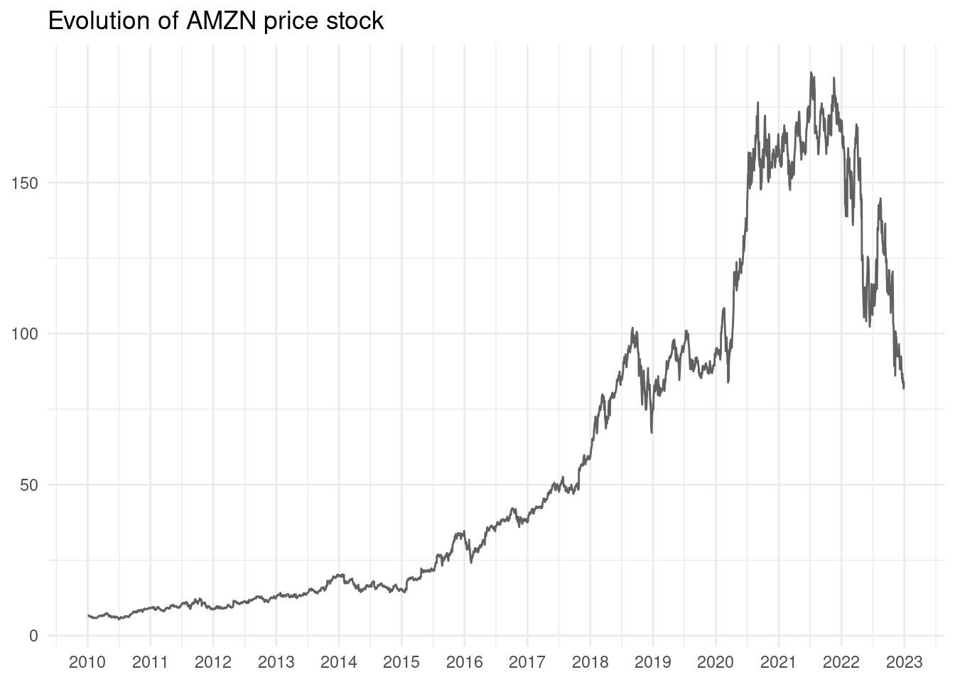
We can pick a narrower range of dates to do the plot. Note that date is in Date format, so boundary values must be presented in that format.
start_date <- as.Date("2022-02-01")
end_date <- as.Date("2022-03-31")
Here is the evolution of Amazon during February and March 2022.
big_tech_stock_prices |>
  filter(stock_symbol == "AMZN", date >= start_date, date <= end_date) |>
  ggplot(aes(date, adj_close)) +
  geom_point() +
  geom_line(color = "#606060") +
  theme_minimal() +
  scale_x_date(name = NULL, date_breaks = "2 weeks") +
  labs(title = "Short-Term Evolution of AMZN", y = NULL)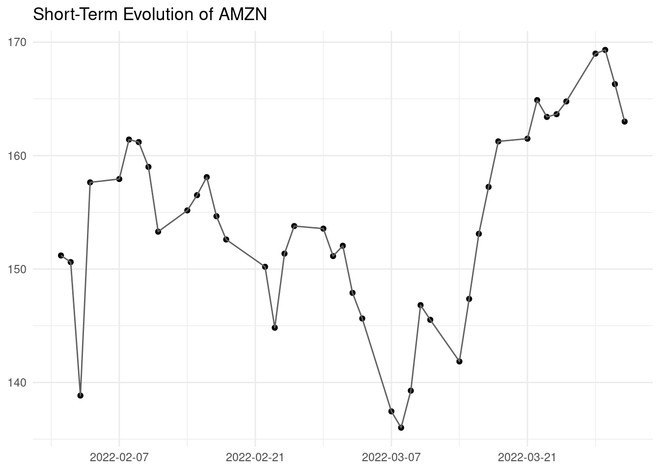
Note that stock prices are not spaced evenly, as we have information for the days where stocks are traded.
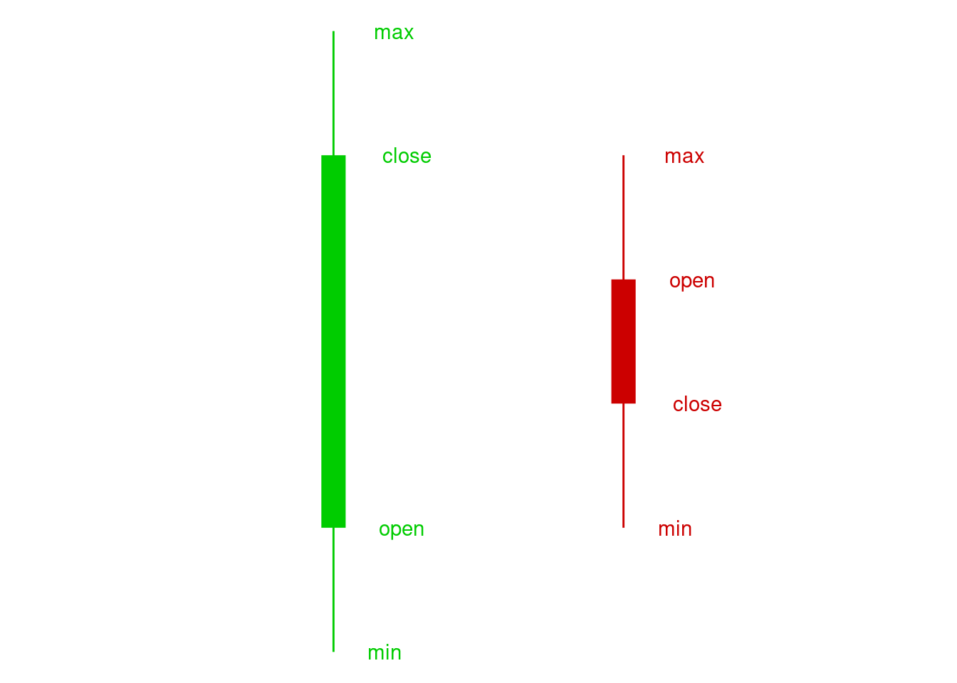
A Candlestick Plot
A candlestick plot is a type of financial chart used to represent the movement of an asset’s price over a specified period of time. It is commonly used in technical analysis to identify patterns and trends in the price behavior of financial instruments such as stocks, commodities, and currencies.
The candlestick plot is composed of a series of rectangular bars, each representing a specific time interval (e.g. a day or an hour). Each bar has body and wicks (also called shadows). The body of the bar represents the opening and closing prices of the asset during that time interval, while the wicks represent the high and low prices reached.
If the closing price is higher than the opening price, the body of the candlestick is typically colored green or white to indicate a bullish market. If the closing price is lower than the opening price, the body of the candlestick is typically colored red or black to indicate a bearish market.
Here is schematic representation of the candlestick plot:
Here is the example of candlestick plot. I am using two geom_segment():
- The wicks of each day are defined in the first segment.
- The body of the plot is presented in the second segment. I have done it ticker doing
linewidth = 2.
To assign the color to each bar, I have defined an ev variable which indicates if the market is bullish with ev = "up" or bearish with ev = "down". The real colors of the plot are defined in the values of scale_color_manual.
big_tech_stock_prices |>
  filter(stock_symbol == "AMZN", date >= start_date, date <= end_date) |>
  mutate(ev = ifelse(open < close, "up", "down")) |>
  ggplot(aes(date, adj_close)) +
  geom_segment(aes(x = date, y = high, xend = date, yend = low, color = ev)) +
  geom_segment(aes(x = date, y = open, xend = date, yend = close, color = ev), linewidth = 2) +
  theme_minimal() +
  theme(legend.position = "none") +
  scale_color_manual(values = c("#CC0000", "#00CC00")) +
  labs(title = "Short-Term Evolution of AMZN", x=NULL, y=NULL)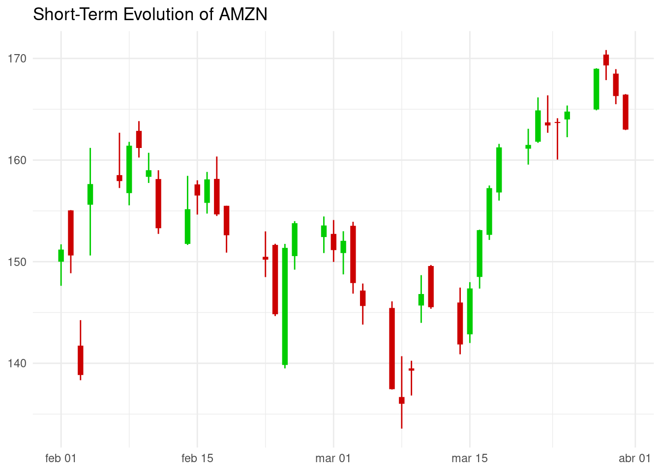
Traders and investors use candlestick charts to analyze patterns and trends in the price movements of financial instruments, with the goal of making more informed trading decisions.
References
plotlywebsite Candlestick Charts in R https://plotly.com/r/candlestick-charts/.- Big Tech Stock Prices, tidytuesday GitHub repo (2023-02-07) https://github.com/rfordatascience/tidytuesday/blob/master/data/2023/2023-02-07/readme.md
- Dancho, Matt (2022). Charting with tidyquant. https://cran.r-project.org/web/packages/tidyquant/vignettes/TQ04-charting-with-tidyquant.html
- Ko Chiu Yu (2020). Techincal Analysis with R (second edition) https://bookdown.org/kochiuyu/technical-analysis-with-r-second-edition2/
All links retrieved on 2023-03-22.
Session Info
## R version 4.2.3 (2023-03-15)
## Platform: x86_64-pc-linux-gnu (64-bit)
## Running under: Linux Mint 21.1
##
## Matrix products: default
## BLAS:   /usr/lib/x86_64-linux-gnu/blas/libblas.so.3.10.0
## LAPACK: /usr/lib/x86_64-linux-gnu/lapack/liblapack.so.3.10.0
##
## locale:
##  [1] LC_CTYPE=es_ES.UTF-8       LC_NUMERIC=C
##  [3] LC_TIME=es_ES.UTF-8        LC_COLLATE=es_ES.UTF-8
##  [5] LC_MONETARY=es_ES.UTF-8    LC_MESSAGES=es_ES.UTF-8
##  [7] LC_PAPER=es_ES.UTF-8       LC_NAME=C
##  [9] LC_ADDRESS=C               LC_TELEPHONE=C
## [11] LC_MEASUREMENT=es_ES.UTF-8 LC_IDENTIFICATION=C
##
## attached base packages:
## [1] stats     graphics  grDevices utils     datasets  methods   base
##
## other attached packages:
##  [1] kableExtra_1.3.4 forcats_0.5.2    stringr_1.5.0    dplyr_1.0.10
##  [5] purrr_1.0.1      readr_2.1.3      tidyr_1.3.0      tibble_3.1.8
##  [9] ggplot2_3.4.0    tidyverse_1.3.2
##
## loaded via a namespace (and not attached):
##  [1] svglite_2.1.1       lubridate_1.9.1     assertthat_0.2.1
##  [4] digest_0.6.31       utf8_1.2.2          R6_2.5.1
##  [7] cellranger_1.1.0    backports_1.4.1     reprex_2.0.2
## [10] evaluate_0.20       highr_0.10          httr_1.4.4
## [13] blogdown_1.16       pillar_1.8.1        rlang_1.0.6
## [16] googlesheets4_1.0.1 readxl_1.4.1        rstudioapi_0.14
## [19] jquerylib_0.1.4     rmarkdown_2.20      labeling_0.4.2
## [22] webshot_0.5.4       googledrive_2.0.0   munsell_0.5.0
## [25] broom_1.0.3         compiler_4.2.3      modelr_0.1.10
## [28] xfun_0.36           pkgconfig_2.0.3     systemfonts_1.0.4
## [31] htmltools_0.5.4     tidyselect_1.2.0    bookdown_0.32
## [34] viridisLite_0.4.1   fansi_1.0.4         crayon_1.5.2
## [37] tzdb_0.3.0          dbplyr_2.3.0        withr_2.5.0
## [40] grid_4.2.3          jsonlite_1.8.4      gtable_0.3.1
## [43] lifecycle_1.0.3     DBI_1.1.3           magrittr_2.0.3
## [46] scales_1.2.1        cli_3.6.0           stringi_1.7.12
## [49] cachem_1.0.6        farver_2.1.1        fs_1.6.0
## [52] xml2_1.3.3          bslib_0.4.2         ellipsis_0.3.2
## [55] generics_0.1.3      vctrs_0.5.2         tools_4.2.3
## [58] glue_1.6.2          hms_1.1.2           fastmap_1.1.0
## [61] yaml_2.3.7          timechange_0.2.0    colorspace_2.1-0
## [64] gargle_1.2.1        rvest_1.0.3         knitr_1.42
## [67] haven_2.5.1         sass_0.4.5