In [a previous post]https://jmsallan.netlify.app/blog/implementation-of-dbscan-clustering-in-r/), I introduced a clustering technique called discrete-based spatial clustering and applications with noise (DBSCAN). This clustering technique is density-based, detecting sets of elements located in a region of high density. This approach is different from traditional clustering techniques like k-means or hierarchical clustering. These techniques identify sets where the distance within elements is smaller than distance between elements of other clusters.

DBSCAN is a suitable technique for spatial analysis. While in distance-based techniques like k-means the regions defined by clusters tend to be circular, DBSCAN clusters can have any shape.

In this post, I will extend the DBSCAN workflow of previous posts in two directions:

• How to identify an adequate value of the distance between core points eps using the plot of k-nearest neighbor distances.
• How to use the functions of the dbscan package with spatial objects, using the distance matrix instead of geographical coordinates.

library(tidyverse) # data handling and plotting
library(sf) # geocomputation
library(BAdatasetsSpatial) # BCN map
library(dbscan) # DBSCAN clustering
library(RColorBrewer) # color palettes

I will be using the dataset of nightlife Barcelona venues nightlife_2024, and its transformation as spatial object nightlife_2024_sf. To plot the final result, I will use the bcn_neigh Barcelona map of neighborhoods.

bcn_neigh <- BCNNeigh |>
  select(c_barri, n_barri, c_distri, n_distri)

nightlife_2024 <- data_2024 |>
  select(nom_local, latitud, longitud, nom_barri, codi_barri)

nightlife_2024_sf <- nightlife_2024 |>
  st_as_sf(coords = c("longitud", "latitud"), crs = 4326, remove = FALSE)

A common approach to cluster spatial data is use longitude and latitude directly, as they represent approximately the \(x\) and \(y\) coordinates of each point. But in DBSCAN the eps parameter is expressed in distance units, so we cannot use longitude and latitude directly. dbscan::dbscan() allows using a distance matrix rather than a set of coordinates. To obtain this distance, I have used the sf::st_distance() function and transformed the result to a distance object with as.dist().

nl_distances <- st_distance(nightlife_2024_sf) |>
  as.dist()

As it is two-dimensional dataset, I will use the standard value minPts = 3. We need, though, to establish an adequate value of maximum distance between contiguous core points eps. To do so, I have used the k-nearest neighbor distances plot. Obtained with dbscan::kNNdistplot(), it represents the distance between each element and its k-th distant neighbor. As minPts includes the point from we calculate distances, we need to set k = minPts - 1.

kNNdistplot(nl_distances, k = 2)
abline(a = 400, b = 0, col = "red", lty = 2)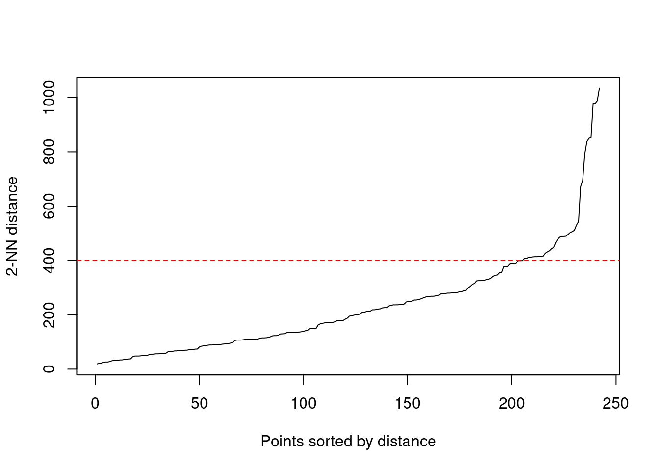

The choice of eps is the elbow point of this plot. In this case, I have chosen eps = 450. The results of the clustering are stored in nl_dbscan.

nl_dbscan <- dbscan(nl_distances, eps = 450, minPts = 3)
table(nl_dbscan$cluster)

## 
##  0  1  2  3  4  5  6  7  8 
## 13 13 85 96  3  4 13  4 11

The algorithm returns eight different clusters and 13 noise points, not assigned to any cluster. These noise points are assigned to the 0 label.

augment(nl_dbscan, nightlife_2024_sf) |>
  filter(noise) |>
  st_drop_geometry() |>
  select(nom_local, .cluster, noise)

## # A tibble: 13 × 3
##    nom_local                 .cluster noise
##    <chr>                     <fct>    <lgl>
##  1 NUMANCIA 12 NIGHT CLUB    0        TRUE 
##  2 LUXOR SHISHA CLUB         0        TRUE 
##  3 SAFARI DISCO CLUB         0        TRUE 
##  4 MAGBA BRUNCH SISHA LOUNGE 0        TRUE 
##  5 LUXIUM LOUNGE CLUB        0        TRUE 
##  6 LOUNGE BAR CHILL OUT      0        TRUE 
##  7 RAKATÁ                    0        TRUE 
##  8 LA CALLE                  0        TRUE 
##  9 CLUB EL NIDO ROJO         0        TRUE 
## 10 DISCOTECA PEDRALBES       0        TRUE 
## 11 LOS TILOS                 0        TRUE 
## 12 DOWNTOWN                  0        TRUE 
## 13 DOWNTOWN                  0        TRUE

To obtain a preliminary plot of the clusters, I have used broom::augment() to assign points to clusters.

augment(nl_dbscan, nightlife_2024) |>
  ggplot(aes(longitud, latitud, color = .cluster)) +
  geom_point() +   
  theme_minimal(base_size = 14)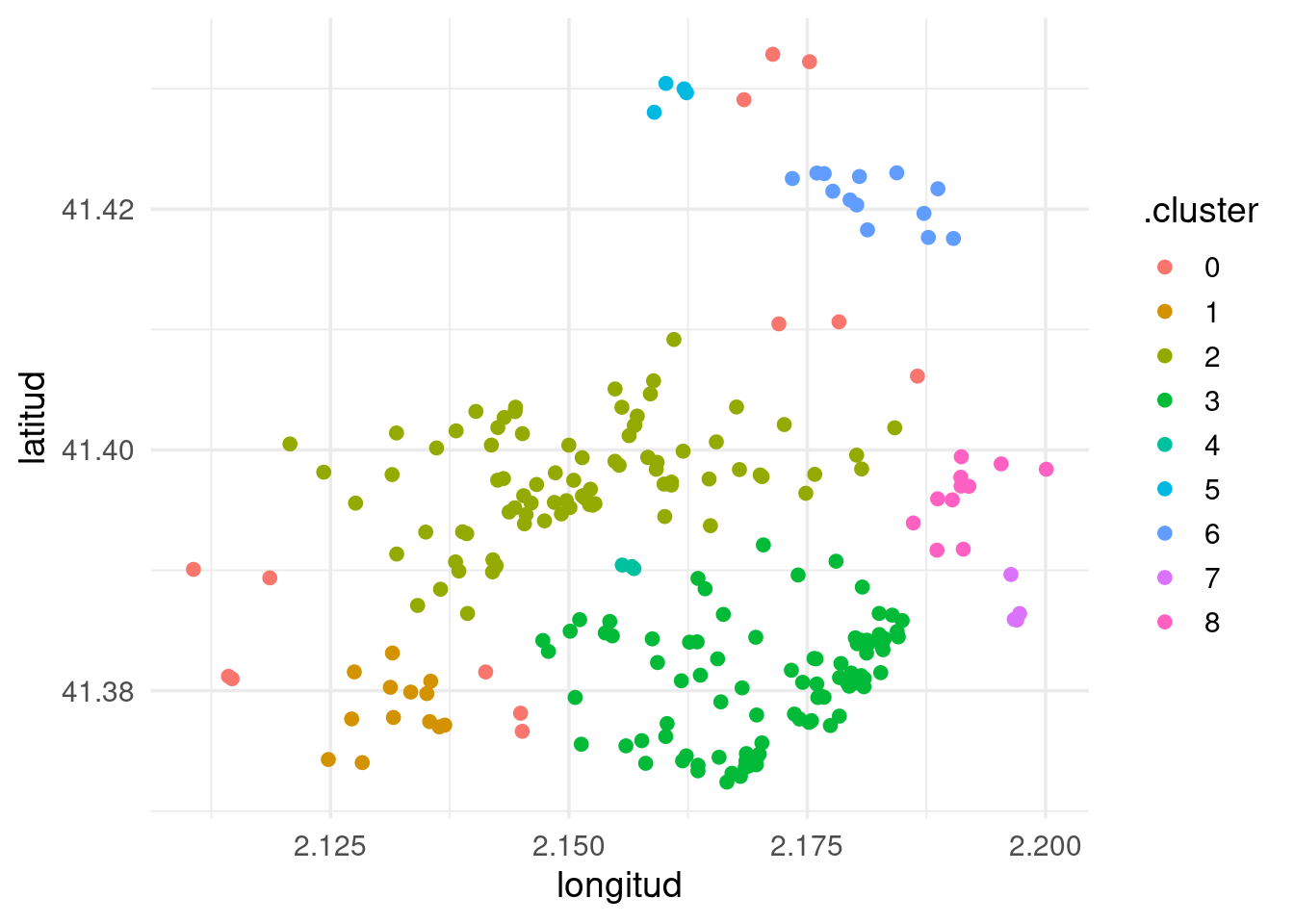

Finally, I can place clusters over a map. I need to take into account two issues:

• We cannot use broom::augment() with spatial objects, so I need to assign clusters with dplyr::mutate().
• I have created a color palette col_clust using the divergent Brewer palette Paired, setting in grey the noise points.

col_clust <- c("#A0A0A0", brewer.pal(8, "Paired"))

nl_dbscan_sf <- nightlife_2024_sf |>
  mutate(cluster = as.factor(nl_dbscan$cluster))

ggplot(bcn_neigh) +
  geom_sf(fill = "white") +
  geom_sf(data = nl_dbscan_sf, aes(color = cluster)) +
  scale_color_manual(values = col_clust) +
  theme_void() +
  theme(legend.position = "bottom")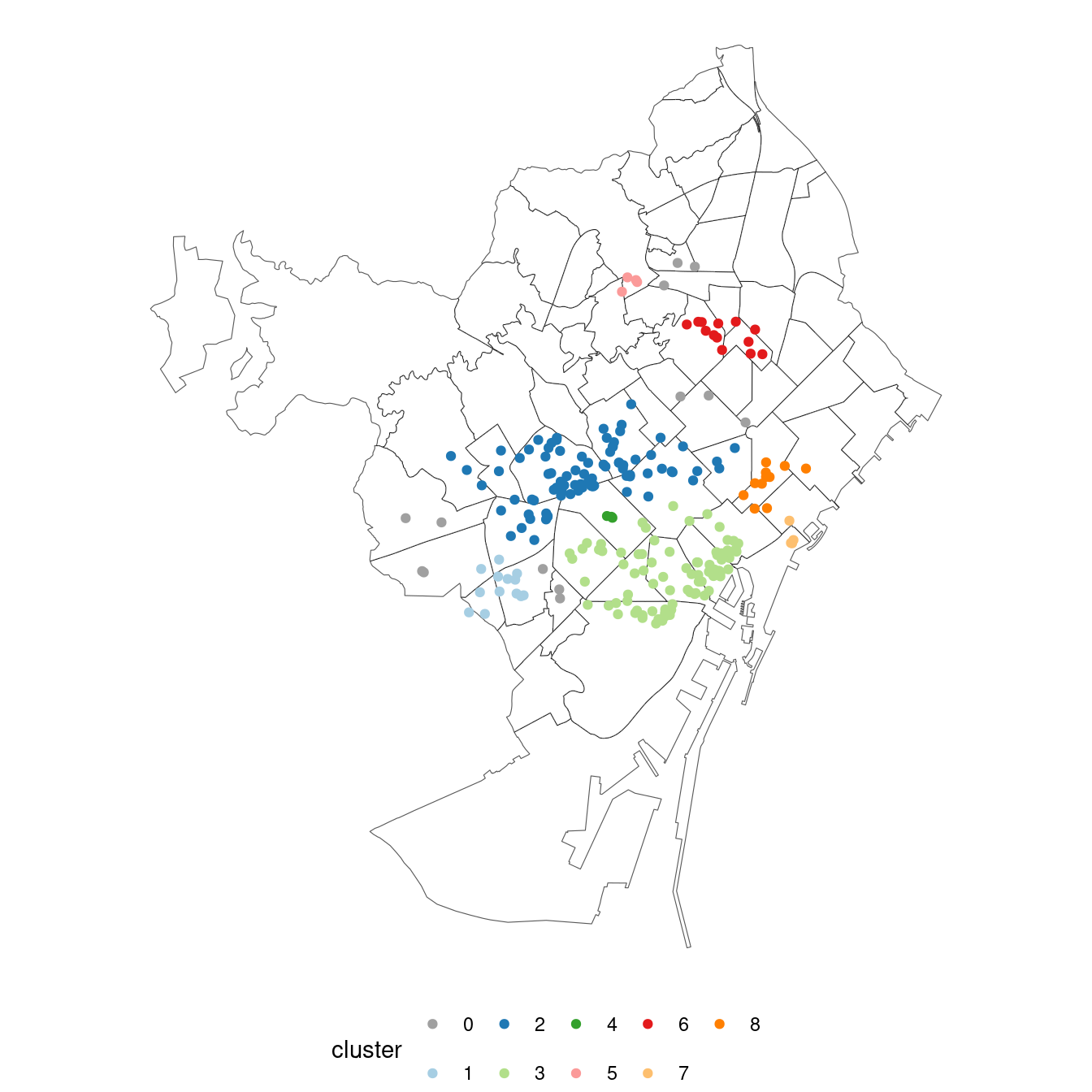

Here is the result of the DBSCAN clustering:

• Two large clusters: cluster 2 corresponds with the city downtown, and 3 with the more residential districts of Gràcia and Sant Gervasi.
• Three medium-size clusters. Cluster 6 is located at the northern neighborhoods, mainly El Guinardó. Cluster 8 includes venues around Poblenou. Cluster 1 includes venues at Sants and Badal.
• Three small clusters, located at Eixample (cluster 4), Vila Olímpica (cluster 7) and Horta (cluster 5).

## R version 4.5.2 (2025-10-31)
## Platform: x86_64-pc-linux-gnu
## Running under: Linux Mint 21.1
## 
## Matrix products: default
## BLAS:   /usr/lib/x86_64-linux-gnu/blas/libblas.so.3.10.0 
## LAPACK: /usr/lib/x86_64-linux-gnu/lapack/liblapack.so.3.10.0  LAPACK version 3.10.0
## 
## locale:
##  [1] LC_CTYPE=es_ES.UTF-8       LC_NUMERIC=C              
##  [3] LC_TIME=es_ES.UTF-8        LC_COLLATE=es_ES.UTF-8    
##  [5] LC_MONETARY=es_ES.UTF-8    LC_MESSAGES=es_ES.UTF-8   
##  [7] LC_PAPER=es_ES.UTF-8       LC_NAME=C                 
##  [9] LC_ADDRESS=C               LC_TELEPHONE=C            
## [11] LC_MEASUREMENT=es_ES.UTF-8 LC_IDENTIFICATION=C       
## 
## time zone: Europe/Madrid
## tzcode source: system (glibc)
## 
## attached base packages:
## [1] stats     graphics  grDevices utils     datasets  methods   base     
## 
## other attached packages:
##  [1] RColorBrewer_1.1-3      dbscan_1.2.3            BAdatasetsSpatial_0.1.0
##  [4] sf_1.0-20               lubridate_1.9.4         forcats_1.0.1          
##  [7] stringr_1.6.0           dplyr_1.1.4             purrr_1.2.0            
## [10] readr_2.1.5             tidyr_1.3.1             tibble_3.3.0           
## [13] ggplot2_4.0.0           tidyverse_2.0.0        
## 
## loaded via a namespace (and not attached):
##  [1] s2_1.1.7           utf8_1.2.4         sass_0.4.10        generics_0.1.3    
##  [5] class_7.3-23       KernSmooth_2.23-26 blogdown_1.21      stringi_1.8.7     
##  [9] hms_1.1.4          digest_0.6.37      magrittr_2.0.4     evaluate_1.0.3    
## [13] grid_4.5.2         timechange_0.3.0   bookdown_0.43      fastmap_1.2.0     
## [17] jsonlite_2.0.0     e1071_1.7-16       DBI_1.2.3          scales_1.4.0      
## [21] jquerylib_0.1.4    cli_3.6.4          rlang_1.1.6        units_0.8-7       
## [25] withr_3.0.2        cachem_1.1.0       yaml_2.3.10        tools_4.5.2       
## [29] tzdb_0.5.0         vctrs_0.6.5        R6_2.6.1           proxy_0.4-27      
## [33] lifecycle_1.0.4    classInt_0.4-11    pkgconfig_2.0.3    pillar_1.11.1     
## [37] bslib_0.9.0        gtable_0.3.6       Rcpp_1.1.0         glue_1.8.0        
## [41] xfun_0.52          tidyselect_1.2.1   rstudioapi_0.17.1  knitr_1.50        
## [45] farver_2.1.2       htmltools_0.5.8.1  labeling_0.4.3     rmarkdown_2.29    
## [49] wk_0.9.4           compiler_4.5.2     S7_0.2.0

References

- Ester, Martin, Hans-Peter Kriegel, Jörg Sander, Xiaowei Xu, et al. (1996). A Density-Based Algorithm for Discovering Clusters in Large Spatial Databases with Noise. In Proceedings of 2nd International Conference on Knowledge Discovery and Data Mining (KDD-96), 226–231. https://dl.acm.org/doi/10.5555/3001460.3001507
- Hahsler, M., Piekenbrock, M., & Doran, D. (2019). dbscan: Fast density-based clustering with R. Journal of Statistical Software, 91, 1-30. https://doi.org/10.18637/jss.v091.i01