Warnings and Episodes of Pollution in Barcelona

Jose M Sallan 2025-07-31 12 min read

One of the tools of exploratory data analysis is handling tidy data to discover patterns in data. In this post, I will illustrate this by examining the preventive warnings and environmental episodes concerning air quality in Barcelona. Throughout the post, I will use the tools of the tidyverse for data handling and visualization.

library(tidyverse)

Our starting point will be a dataset of air quality measurement stations and of hourly observations of level of pollutants from these stations. Both datasets have been obtained from the Open Data BCN portal.

Here is the listing of stations:

estacions

##   estacio                    nom_cabina longitud  latitud codi_districte
## 1      50        Barcelona - Ciutadella   2.1874 41.38640              1
## 2      43          Barcelona - Eixample   2.1538 41.38530              5
## 3      44            Barcelona - Gràcia   2.1534 41.39870              6
## 4      57       Barcelona - Palau Reial   2.1151 41.38750              4
## 5       4          Barcelona - Poblenou   2.2045 41.40390             10
## 6      42             Barcelona - Sants   2.1331 41.37880              3
## 7      54       Barcelona - Vall Hebron   2.1480 41.42610              7
## 8      58 Barcelona - Observatori Fabra   2.1239 41.41843              5
##   codi_barri       nom_estacio
## 1          4        Ciutadella
## 2          9          Eixample
## 3         31            Gràcia
## 4         21       Palau Reial
## 5         68          Poblenou
## 6         18             Sants
## 7         41       Vall Hebron
## 8         22 Observatori Fabra

And the air quality data. The dataset covers the period 2018-2025 and the NO2 and PM10 pollutants.

aq

## # A tibble: 796,797 × 8
##    station pollutant datetime             year month   day  hour value
##      <dbl>     <dbl> <dttm>              <dbl> <dbl> <dbl> <dbl> <dbl>
##  1      50         8 2025-07-27 01:00:00  2025     7    27     1    11
##  2      50         8 2025-07-27 02:00:00  2025     7    27     2    10
##  3      50         8 2025-07-27 03:00:00  2025     7    27     3    15
##  4      50         8 2025-07-27 04:00:00  2025     7    27     4    10
##  5      50         8 2025-07-27 05:00:00  2025     7    27     5     6
##  6      50         8 2025-07-27 06:00:00  2025     7    27     6     9
##  7      50         8 2025-07-27 07:00:00  2025     7    27     7    22
##  8      50         8 2025-07-27 08:00:00  2025     7    27     8    18
##  9      50         8 2025-07-27 09:00:00  2025     7    27     9     9
## 10      50         8 2025-07-27 10:00:00  2025     7    27    10     6
## # ℹ 796,787 more rows

To facilitate data handling I will modify the aq dataset:

Adding the station name nom_estacio.
Obtaining the date from datetime.

aq <- aq |>
  left_join(estacions |> select(estacio, nom_estacio), by = c("station" = "estacio")) |>
  mutate(date = as_date(datetime))

Preventive Warnings

A preventive warning for air pollution is issued when:

The hourly average of NO2 at one of the air quality monitoring stations exceeds 160 µg/m³ and the 24-hour forecast does not indicate an improvement in NO2 levels.
The daily average of PM10 from the previous day exceeds 50 µg/m³ at more than one air quality monitoring station, and the 24-hour forecast does not indicate an improvement in PM10 levels.

Let’s start examining the NO2 warnings. The values of NO2 are obtained filtering by pollutant == 8. As we will see later, values of NO2 higher than 200 correspond to an environmental episode, so I am filtering by values between 160 and 200

aq |>
  filter(pollutant == 8) |>
  filter(value >= 160, value < 200) |>
  arrange(datetime) |>
  select(nom_estacio, date, hour, value) |>
  print(n = Inf)

## # A tibble: 23 × 4
##    nom_estacio date        hour value
##    <chr>       <date>     <dbl> <dbl>
##  1 Gràcia      2018-06-21    10   164
##  2 Eixample    2018-06-21    11   197
##  3 Gràcia      2018-06-21    11   165
##  4 Sants       2018-06-21    12   165
##  5 Eixample    2018-06-21    12   160
##  6 Eixample    2018-06-22    10   167
##  7 Eixample    2018-08-03    10   169
##  8 Eixample    2019-01-25    10   173
##  9 Gràcia      2019-01-25    10   168
## 10 Gràcia      2019-01-25    11   165
## 11 Eixample    2019-06-27    10   172
## 12 Gràcia      2019-06-27    20   164
## 13 Gràcia      2019-06-28     9   173
## 14 Vall Hebron 2019-06-28    11   181
## 15 Gràcia      2019-06-29    10   166
## 16 Eixample    2019-06-29    11   185
## 17 Gràcia      2019-06-29    11   165
## 18 Gràcia      2019-09-18    11   172
## 19 Sants       2019-11-20    23   160
## 20 Ciutadella  2022-01-28    12   167
## 21 Gràcia      2022-03-31    12   160
## 22 Gràcia      2023-06-19     9   161
## 23 Gràcia      2023-06-19    15   164

These are the measures between 160 and 200 of NO2 between 2018 and 2025. Let’s arrange them in a wide table with tidyr::pivot:wider().

aq |>
  filter(pollutant == 8) |>
  filter(value >= 160, value < 200) |>
  group_by(date, nom_estacio) |>
  count() |>
  pivot_wider(values_from = n, names_from = nom_estacio, values_fill = 0)

## # A tibble: 12 × 6
## # Groups:   date [12]
##    date       Eixample Gràcia Sants `Vall Hebron` Ciutadella
##    <date>        <int>  <int> <int>         <int>      <int>
##  1 2018-06-21        2      2     1             0          0
##  2 2018-06-22        1      0     0             0          0
##  3 2018-08-03        1      0     0             0          0
##  4 2019-01-25        1      2     0             0          0
##  5 2019-06-27        1      1     0             0          0
##  6 2019-06-28        0      1     0             1          0
##  7 2019-06-29        1      2     0             0          0
##  8 2019-09-18        0      1     0             0          0
##  9 2019-11-20        0      0     1             0          0
## 10 2022-01-28        0      0     0             0          1
## 11 2022-03-31        0      1     0             0          0
## 12 2023-06-19        0      2     0             0          0

We have detected twelve preventive warnings from excess of NO2, spanning from 2018 to 2023. There were no NO2 warnings in 2024 and 2025. These excess of NO2 was registered in five oot of eight measurement stations.

Let’s examine now the preventive warnings form PM10. These correspond with average daily values of PM10 detected in more than one station on the same day. Let’s start picking these values in a pm10_50 table. To build it I have:

computed the average daily value grouping by date and station name nom_estacio.
filtered the average daily values of PM10 between 50 and 80.

pm10_50 <- aq |>
  filter(pollutant == 10) |>
  group_by(date, nom_estacio) |>
  summarise(pm10 = mean(value, na.rm = TRUE), .groups = "drop") |>
  filter(pm10 >= 50, pm10 < 80)

Now I want to obtain the dates when there were moderatelly abnormal values of PM10 in more than one station. As I want to know the stations where measures took place, I am using dplyr::mutate() together with dplyr::group_b(). The column n has the number of affected stations, repeated for each date. Finally, I filter by values of n greater than one.

pm10_50_more1 <- pm10_50 |>
  group_by(date) |>
  mutate(n = n()) |>
  ungroup() |>
  filter(n > 1)

The resulting table has 109 rows, so the warnings from PM10 are more frequent than from NO2. Let’s examine two possible patters:

Month of appearance of the warning.
Stations involved in the warning.

When building the plot of months, I see than some months have no warnings. To account for this, I am creating a months tibble.

months <- tibble(num_month = 1:12, month = c("jan", "feb", "mar", "apr", "may", "jun", "jul", "aug", "sep", "oct", "nov", "dec"))

And here is the plot of occurrences of warnings by month. Observe the use of the month variable as a factor to create the plot.

pm10_50_more1 |>
  mutate(num_month = month(date)) |>
  group_by(num_month) |>
  summarise(n = n(), .groups = "drop") |>
  full_join(months, by = "num_month") |>
  mutate(n = ifelse(is.na(n), 0, n)) |>
  mutate(month = factor(month, levels = months$month)) |>
  ggplot(aes(month, n)) +
  geom_col() +
  theme_minimal(base_size = 12) +
  labs(x = NULL, y = NULL, title = "PM10 warnings by month (2018-2025)")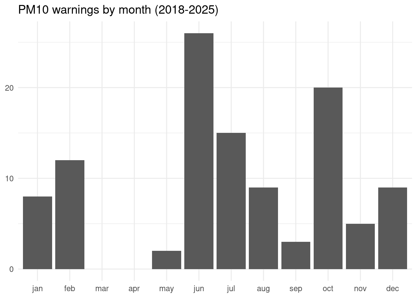

The pattern of occurrences of warnings from PM10 over time is strange: no warnings in March and April, peak values in June and October.

Here is the plot of stations:

pm10_50_more1 |>
  group_by(nom_estacio) |>
  summarise(n = n(), .groups = "drop") |>
  mutate(nom_estacio2 = fct_reorder(nom_estacio, n)) |>
  ggplot(aes(n, nom_estacio2)) +
  geom_col() +
  theme_minimal(base_size = 12) +
  labs(x = NULL, y = NULL, title = "PM10 warnings by station (2018-2025)")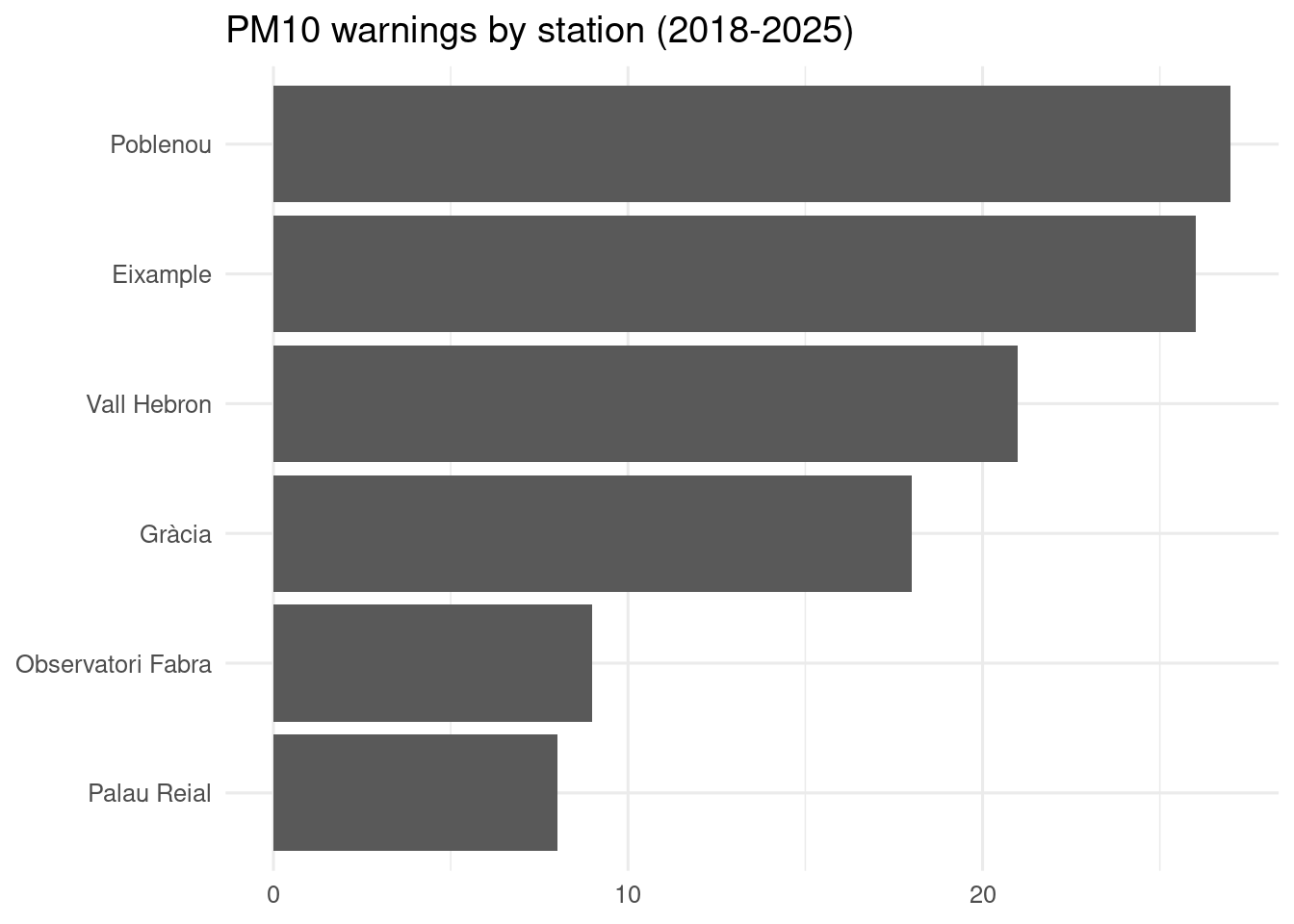

These results make more sense. Poblenou and Vall Hebron are close to the road rings (Ronda Litoral and Ronda de Dalt, respectively), with heavy traffic. Eixample and Gràcia are the among the most populated, also with high values of traffic.

Environmental Episodes

An environmental episode due to high pollution is declared when:

The hourly average of NO₂ exceeds 200 µg/m³ at more than one air quality monitoring station, or when another justified situation requires it.
The daily average of PM₁₀ from the previous day exceeds 80 µg/m³ at more than one air quality monitoring station, and the 24-hour forecast does not indicate an improvement in PM₁₀ levels.
The daily average of PM₁₀ exceeds 50 µg/m³ for three consecutive days at more than one air quality monitoring station, and the 24-hour forecast does not indicate an improvement in PM₁₀ levels.

From the previous analysis, we can guess that environmental episodes from excess of NO2 will be scarce:

aq |>
  filter(pollutant == 8) |>
  filter(value >= 200) |>
  select(nom_estacio, date, datetime, value)

## # A tibble: 5 × 4
##   nom_estacio date       datetime            value
##   <chr>       <date>     <dttm>              <dbl>
## 1 Ciutadella  2019-10-30 2019-10-30 12:00:00   216
## 2 Eixample    2019-06-28 2019-06-28 10:00:00   202
## 3 Eixample    2019-06-28 2019-06-28 11:00:00   207
## 4 Gràcia      2019-06-28 2019-06-28 10:00:00   213
## 5 Gràcia      2019-06-28 2019-06-28 11:00:00   233

In the period 2018-2025, there were environmental episodes by excess of NO2 on 28 June and 20 October of 2019.

There are two possible reasons of preventing warning from excess of PM10. Let’s examine first events where PM10 was higher than 80 in more than one station, proceeding in a similar way as with the warnings. The pm10_80 table contains average daily values higher than 80.

pm10_80 <- aq |>
  filter(pollutant == 10) |>
  group_by(date, nom_estacio) |>
  summarise(pm10 = mean(value, na.rm = TRUE), .groups = "drop") |>
  filter(pm10 >= 80)

In pm10_80_more1 we retain the days with values above 80 in more than one station.

pm10_80_more1 <- pm10_80 |>
  group_by(date) |>
  mutate(n = n()) |>
  ungroup() |>
  filter(n > 1)

This table has 35 rows so this is not a frequent event. Let’s examine the days with environmental episodes:

pm10_80_more1 |>
  group_by(date) |>
  summarise(n = n(), .groups = "drop")

## # A tibble: 8 × 2
##   date           n
##   <date>     <int>
## 1 2018-06-24     2
## 2 2019-12-17     6
## 3 2019-12-18     6
## 4 2020-01-24     5
## 5 2020-10-21     3
## 6 2020-10-22     2
## 7 2021-02-06     6
## 8 2021-02-22     5

There were eight days with average daily values of PM10 higher than 80 in more than one station. The most acute episodes were on 17 and 18 December 2019 and 2 of June 2021, when abnormally high values of PM10 were registered in six stations.

We can have an environmental episode from PM10 when average daily values of PM10 are observed in more than one station three days in a row. To detect this, we use the dplyr::lag() function which gives is the value of the previous day pm10_1 and of the day before pm10_2. The episodes are detected with the three_days variable.

aq |>
  filter(pollutant == 10) |>
  group_by(date, nom_estacio) |>
  summarise(pm10 = mean(value, na.rm = TRUE), .groups = "drop") |>
  arrange(nom_estacio, date) |>
  mutate(pm10_1 = lag(pm10),
         pm10_2 = lag(pm10, 2)) |>
  mutate(three_days = pm10 >= 50 & pm10_1 >= 50 & pm10_2 >= 50) |>
  filter(three_days) |>
  group_by(date) |>
  mutate(n = n()) |>
  ungroup() |>
  filter(n > 1) |>
  arrange(date, nom_estacio) |>
  select(date, nom_estacio, pm10:pm10_2)

## # A tibble: 8 × 5
##   date       nom_estacio  pm10 pm10_1 pm10_2
##   <date>     <chr>       <dbl>  <dbl>  <dbl>
## 1 2019-12-19 Eixample     61.1  104.   100. 
## 2 2019-12-19 Gràcia       59.9  102.    96.2
## 3 2019-12-19 Poblenou     65.1  102.    95.0
## 4 2019-12-19 Vall Hebron  60.2  106.    94.6
## 5 2020-01-24 Eixample    103.    51.2   50.4
## 6 2020-01-24 Poblenou     93.8   67.5   55.1
## 7 2022-10-20 Eixample     85.0   88.2   70  
## 8 2022-10-20 Gràcia       63.9   64.9   52.4

The days detected with this episode are:

17 to 19 December 2019. 18 and 19 December 2019 had also environmental episodes as there were values of PM10 above 80 in more than one station.
22 to 24 January 2020, affecting Eixample and Poblenou.
18 to 20 October 2022. This is the last environmental episode so far, affecting Eixample and Gracia.

Warnings and Episodes of Pullution in Barcelona

We have detected the preventive warnings and environmental episodes from air pollution in Barcelona. We have observed that the warnings and episodes from PM10 were much more frequent than from NO2. It is to notice that there have not been environmental episodes from PM10 and NO2 since 2022. This means that the measures to improve air quality in Barcelona have been effective. Regarding preventive warnings, the most recent have been in June 2025 and November 2024.

pm10_50_more1 |>
  filter(year(date) >= 2024) |>
  group_by(date) |>
  summarise(n = n(), .groups = "drop")

## # A tibble: 4 × 2
##   date           n
##   <date>     <int>
## 1 2024-11-25     5
## 2 2024-12-19     5
## 3 2025-06-20     2
## 4 2025-06-24     2

References

Air quality data from the measure stations of the city of Barcelona https://opendata-ajuntament.barcelona.cat/data/en/dataset/qualitat-aire-detall-bcn
Air quality measure stations of the city of Barcelona https://opendata-ajuntament.barcelona.cat/data/en/dataset/qualitat-aire-estacions-bcn
Generalitat de Catalunya. ¿Qué es un episodio ambiental? Definición. https://mediambient.gencat.cat/es/05_ambits_dactuacio/atmosfera/qualitat_de_laire/qualitat-de-laire-a-la-conurbacio-de-barcelona/pla_millora_qua_aire_2011_2015/mesures-del-pamqa/episodis_ambientals/definicio/index.html

Session Info

## R version 4.5.1 (2025-06-13)
## Platform: x86_64-pc-linux-gnu
## Running under: Linux Mint 21.1
## 
## Matrix products: default
## BLAS:   /usr/lib/x86_64-linux-gnu/blas/libblas.so.3.10.0 
## LAPACK: /usr/lib/x86_64-linux-gnu/lapack/liblapack.so.3.10.0  LAPACK version 3.10.0
## 
## locale:
##  [1] LC_CTYPE=es_ES.UTF-8       LC_NUMERIC=C              
##  [3] LC_TIME=es_ES.UTF-8        LC_COLLATE=es_ES.UTF-8    
##  [5] LC_MONETARY=es_ES.UTF-8    LC_MESSAGES=es_ES.UTF-8   
##  [7] LC_PAPER=es_ES.UTF-8       LC_NAME=C                 
##  [9] LC_ADDRESS=C               LC_TELEPHONE=C            
## [11] LC_MEASUREMENT=es_ES.UTF-8 LC_IDENTIFICATION=C       
## 
## time zone: Europe/Madrid
## tzcode source: system (glibc)
## 
## attached base packages:
## [1] stats     graphics  grDevices utils     datasets  methods   base     
## 
## other attached packages:
##  [1] lubridate_1.9.4 forcats_1.0.0   stringr_1.5.1   dplyr_1.1.4    
##  [5] purrr_1.0.4     readr_2.1.5     tidyr_1.3.1     tibble_3.2.1   
##  [9] ggplot2_3.5.2   tidyverse_2.0.0
## 
## loaded via a namespace (and not attached):
##  [1] gtable_0.3.6      jsonlite_2.0.0    compiler_4.5.1    tidyselect_1.2.1 
##  [5] jquerylib_0.1.4   scales_1.3.0      yaml_2.3.10       fastmap_1.2.0    
##  [9] R6_2.6.1          labeling_0.4.3    generics_0.1.3    knitr_1.50       
## [13] bookdown_0.43     munsell_0.5.1     bslib_0.9.0       pillar_1.10.2    
## [17] tzdb_0.5.0        rlang_1.1.6       utf8_1.2.4        stringi_1.8.7    
## [21] cachem_1.1.0      xfun_0.52         sass_0.4.10       timechange_0.3.0 
## [25] cli_3.6.4         withr_3.0.2       magrittr_2.0.3    digest_0.6.37    
## [29] grid_4.5.1        rstudioapi_0.17.1 hms_1.1.3         lifecycle_1.0.4  
## [33] vctrs_0.6.5       evaluate_1.0.3    glue_1.8.0        farver_2.1.2     
## [37] blogdown_1.21     colorspace_2.1-1  rmarkdown_2.29    tools_4.5.1      
## [41] pkgconfig_2.0.3   htmltools_0.5.8.1

The Jose M Sallan static website