A Simple Example

Let’s illustrate the Monte Carlo method by examining a lottery presented by Kiehl Dang. Here is the problem definition:

To win a certain lotto, a person must spell the word big. Sixty percent of the tickets contain the letter b, 30% contain the letter i, and 10% contain the letter g. Find the average number of tickets a person must buy to win the prize.

We need to identify uncertainties. These are the values of the tickets, which follow the probability law expressed in the statement.

Then we need to generate random inputs. Let’s write a R function to do this:

run_big <- function(p1 = 0.6, p2 = 0.3){
  
  tickets <- runif(1)
  success <- FALSE
  
  while(!success){
    
    b <- any(tickets <= p1)
    i <- any(tickets > p1 & tickets <= p1 + p2)
    g <- any(tickets > p1 + p2)
    
    if(all(c(b, i, g))){
      success <- TRUE
    }else(
      tickets <- c(tickets, runif(1))
    )
  }
  
  return(length(tickets))
}

The function has two parameters: the probability of getting a ticket with letter b p1, and the probability of getting a ticket with letter i p2. The probability of getting a g is equal to 1 - p1 - p2. The function builds a vector of tickets until it contains all three letters: when this happens it exits the loop making success = TRUE. The function uses runif() to generate a random number for each ticket. The function returns the length of tickets, which is the required number of tickets to obtain the three letters.

Once defined the function, we can run the simulations using the sapply() iterator. Here I am saving the values of the one thousand runs in the trials vector.

set.seed(1111)
trials <- sapply(1:1000, \(x) run_big())

Now it is time to analyze results. Let’s check the mean value of required tickets:

mean(trials)

## [1] 10.584

The obtained value is close to the obtained by Kiehl Dang with a large values of trials.

When performing a Monte Carlo simulation, we are not only interested in the mean value, but also in the probability distribution. Let’s examine the values obtained from the simulation with an histogram.

hist(trials)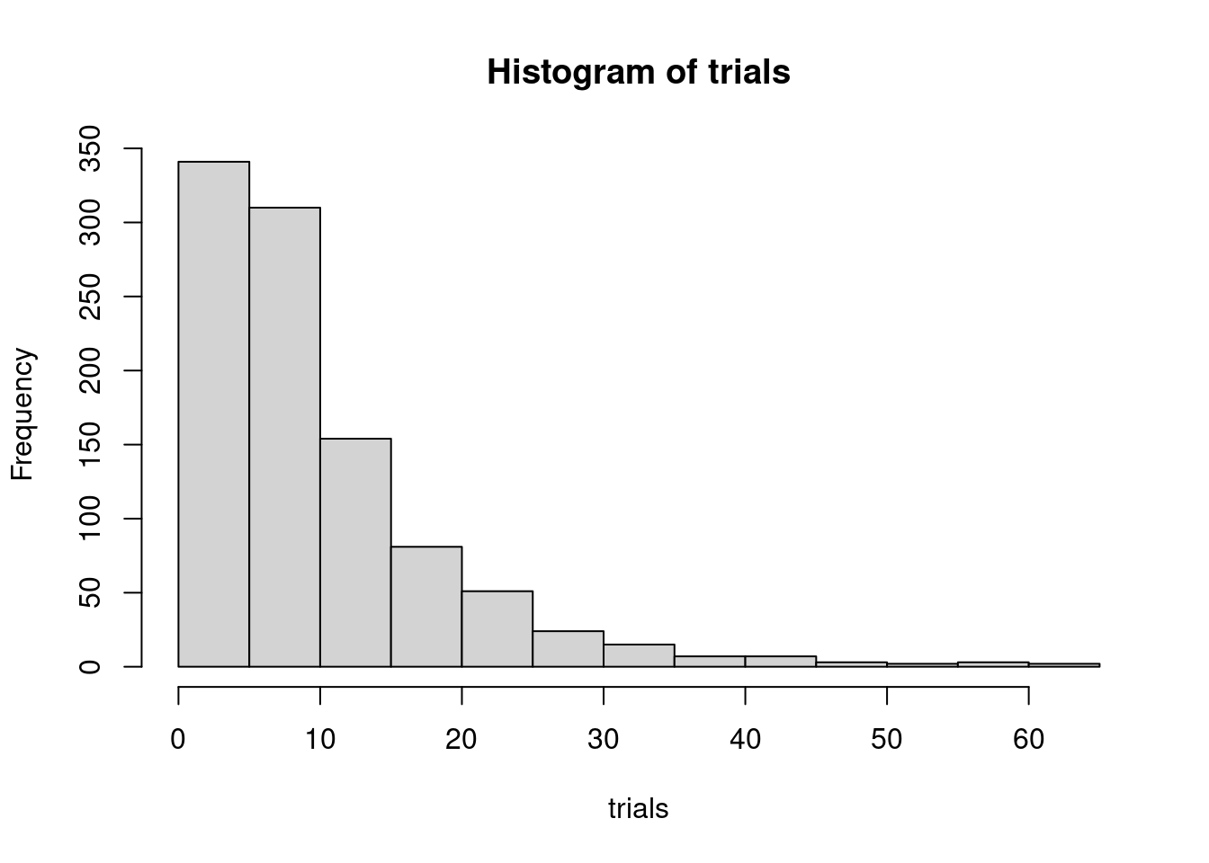

While in most cases we get the three letters with a small number of tickets, sometimes we need to buy many of them to get the three letters: we have a fat tailed distribution. Let’s use the quantile() function to evaluate risks.

quantile(trials, seq(0, 1, 0.1))

##   0%  10%  20%  30%  40%  50%  60%  70%  80%  90% 100% 
##  3.0  3.0  4.0  5.0  6.0  8.0 10.0 12.0 15.0 21.1 63.0

Here we observe that although the mean value of trials is around eleven, there is a probability of 10% of needing to buy 21 tickets or more to obtain the three letters.

The run_big() function allows modifying the probability values of each letter. Intuitively, it seems that the more balanced the probabilities, the less tickets we will need to buy. We can check this running the function with p1 = 1/3 and p2 = 1/3.

set.seed(1313)
trials_balanced <- sapply(1:1000, \(x) run_big(p1 = 1/3, p2  = 1/3))

The mean number of tickets is now:

mean(trials_balanced)

## [1] 5.633

And the probability distribution:

hist(trials_balanced)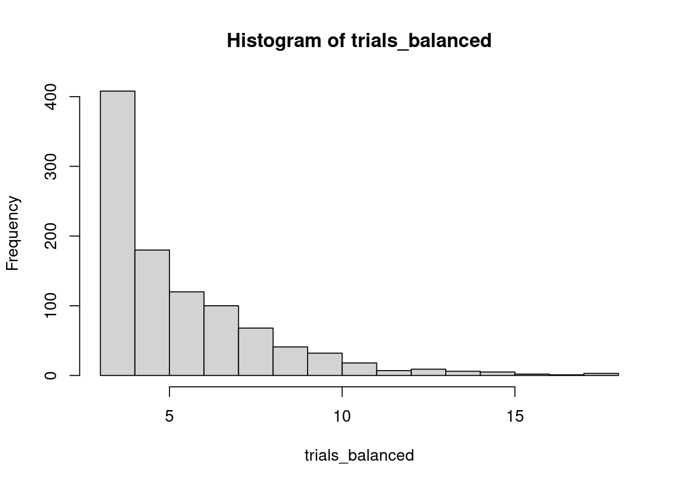

We observe now that the average number of required tickets is much smaller than in the previous case, and that the extreme values are also smaller:

quantile(trials_balanced, seq(0, 1, 0.1))

##   0%  10%  20%  30%  40%  50%  60%  70%  80%  90% 100% 
##    3    3    3    4    4    5    6    6    7    9   18

While in the previous case of unbalanced probabilities we have a small but relevant probability of needing to buy 21 tickets or more, this event is quite unlikely when probabilities are balanced. Therefore, we have confirmed our intuition.

The Monte Carlo Simulation

Monte Carlo simulation is particularly valuable because it helps to account for the variability and randomness in real-world scenarios of processes too complex to be modeled exactly, providing a more robust understanding of potential risks and outcomes. When running a Monte Carlo simulation, we need to pay attention not only to central tendency statistics like mean or median, but also to the overall probability distribution.

References

• Dang, Kiehl (2022). Monte Carlo simulation in R (Detailed code explanation)— Lottery Winner. https://bit.ly/MCLottery
• Monte Carlo method at Wikipedia. https://en.wikipedia.org/wiki/Monte_Carlo_method

The introduction to the Monte Carlo simulation method is an edition of a ChatGPT rendering.

Session Info

## R version 4.4.1 (2024-06-14)
## Platform: x86_64-pc-linux-gnu
## Running under: Linux Mint 21.1
## 
## Matrix products: default
## BLAS:   /usr/lib/x86_64-linux-gnu/blas/libblas.so.3.10.0 
## LAPACK: /usr/lib/x86_64-linux-gnu/lapack/liblapack.so.3.10.0
## 
## locale:
##  [1] LC_CTYPE=es_ES.UTF-8       LC_NUMERIC=C              
##  [3] LC_TIME=es_ES.UTF-8        LC_COLLATE=es_ES.UTF-8    
##  [5] LC_MONETARY=es_ES.UTF-8    LC_MESSAGES=es_ES.UTF-8   
##  [7] LC_PAPER=es_ES.UTF-8       LC_NAME=C                 
##  [9] LC_ADDRESS=C               LC_TELEPHONE=C            
## [11] LC_MEASUREMENT=es_ES.UTF-8 LC_IDENTIFICATION=C       
## 
## time zone: Europe/Madrid
## tzcode source: system (glibc)
## 
## attached base packages:
## [1] stats     graphics  grDevices utils     datasets  methods   base     
## 
## loaded via a namespace (and not attached):
##  [1] digest_0.6.35     R6_2.5.1          bookdown_0.39     fastmap_1.1.1    
##  [5] xfun_0.43         blogdown_1.19     cachem_1.0.8      knitr_1.46       
##  [9] htmltools_0.5.8.1 rmarkdown_2.26    lifecycle_1.0.4   cli_3.6.2        
## [13] sass_0.4.9        jquerylib_0.1.4   compiler_4.4.1    highr_0.10       
## [17] rstudioapi_0.16.0 tools_4.4.1       evaluate_0.23     bslib_0.7.0      
## [21] yaml_2.3.8        jsonlite_1.8.8    rlang_1.1.3