library(purrr)
library(tidygraph)
library(ggraph)
library(gridExtra)
library(patchwork)
The travelling salesman problem (TSP) is a classical optimization problem in graphs consisting in finding the cycle that visits each node exactly once of minimal total distance. It is a classical problem in operations research and it has been tackled with many approaches, including local search algorithms.
A classical neighborhood definition to implement local search algorithms is the 2-opt move. This move consists in picking a pair of non contiguous edges, and rearrange the connections between the four nodes of the two edges as presented in the following example.
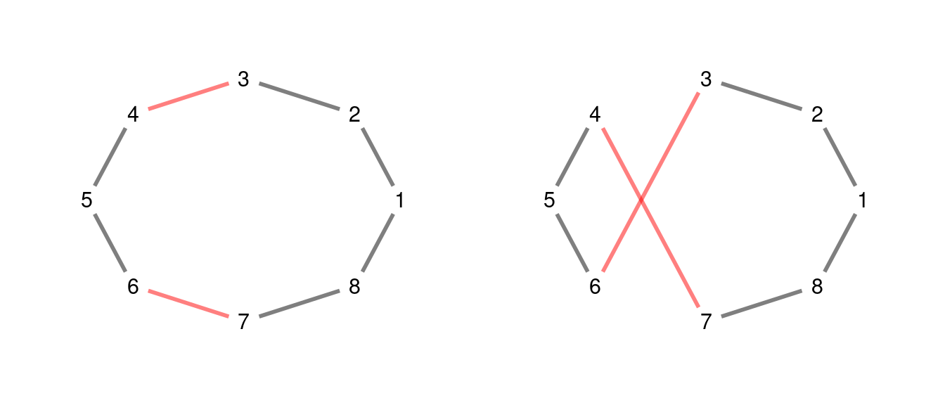
The cycle of the right can be obtained from the cycle on the left reversing the \(\{4,5,6\}\) sequence, so we can label this move as \((4,6)\).
In this post, we will cover some topics related with the 2-opt move
- How many different 2-opt moves exist in a TSP instance of size
n? - How can we generate all possible 2-opt moves for a solution?
- How can we calculate in a fast way the total distance of the cycle resulting from a 2-opt move?
- How can we evaluate total distance for all 2-opt moves of a solution, and choose the move that best improves total distance.
Let’s see how can ask these questions with the R programming language extended by the tidyverse. I will be using the following packages:
- The
purrrfor iterating effectively. - The
tidygraphandggraphpackages to handle and visualize network data. - The
gridExtraandpatchworkpackages to present visualizations on a grid.
Except from purrr, the packages have been used to present figures of 2-opt moves. They have been loaded previously to allow plotting the above figure.
Number of 2-opt Moves
To find the number of 2-opt possible moves, we need to consider that the edges involved in the node must have different nodes. For each of the \(n\) edges of a cycle covering all nodes, only \(n-3\) edges have this property, as we need to exclude the edge itself and the two edges sharing a node with the considered edge. This leads to \(n(n-3)\) possible moves.
But if the problem is symmetric, each 2-opt move has another move yielding the same effect. For the plot above, the \((4, 6)\) move is equivalent to the \((3, 7)\) move. Therefore, the total number of 2-opt moves in a symmetric TSP instance of size \(n\) is \(n(n-3)/2\).
Generating 2-opt Moves
The function move_2opt_table() generates all 2-opt moves for a symmetric TSP in the following way:
- We generate the
edgesdata frame with the positions of node edges(i. j)of a solution. - For each edge, I find all edges
e2with no common nodes for each edgee1. Then, I obtain theielement as the second node of the first edge, andjas the first node of the second edge. - Finally, I choose moves with
i > jto pick those moves with sequences to revert not including the first node.
move_2opt_table <- function(n){

  edges <- data.frame(edge = 1:n, i = 1:n, j = c(2:n, 1))
  e1 <- rep(1:n, each = n-3)
  e2 <- c(sapply(1:n, \(i) ((i+1):(i+n-3) %% n) + 1))

  moves <- data.frame(e1 = e1, e2 = e2, i = e1+1, j = e2)

  moves <- moves[which(moves$i < moves$j), 3:4]

  return(moves)
}
The function is encoded in R base, so there is no additional package to use it.
Here is the result for n = 7…
move_2opt_table(7)## i j
## 1 2 3
## 2 2 4
## 3 2 5
## 4 2 6
## 5 3 4
## 6 3 5
## 7 3 6
## 8 3 7
## 9 4 5
## 10 4 6
## 11 4 7
## 13 5 6
## 14 5 7
## 17 6 7… and the result for n = 8:
move_2opt_table(8)## i j
## 1 2 3
## 2 2 4
## 3 2 5
## 4 2 6
## 5 2 7
## 6 3 4
## 7 3 5
## 8 3 6
## 9 3 7
## 10 3 8
## 11 4 5
## 12 4 6
## 13 4 7
## 14 4 8
## 16 5 6
## 17 5 7
## 18 5 8
## 21 6 7
## 22 6 8
## 26 7 8Obtanining 2-opt Moves
The moves selected by move_2opt_table() reverse sequences that do not contain the first node. This makes the coding of move_2opt() simpler, as we need to care only for the case where \(j\) is equal to the \(n\)-eth node.
move_2opt <- function(vec, i, j, n){
  if(j == n)
    v <- vec[c(1:(i-1), j:i)]
  else
    v <- vec[c(1:(i-1), j:i, (j+1):n)]
  return(v)
}
Here is the move \((4,6)\) of the solution \(\{1,2,3,4,5,6,7,8\}\), presented in the figure above.
move_2opt(1:8, 4, 6, 8)## [1] 1 2 3 6 5 4 7 8We can use the purrr::pmap() function to iterate along the table of 2-opt moves and obtain all solutions as a list.
n <- 6
moves_6 <- move_2opt_table(n)
pmap(moves_6, ~  move_2opt(vec = 1:n, .x, .y, n = n))
## [[1]]
## [1] 1 3 2 4 5 6
##
## [[2]]
## [1] 1 4 3 2 5 6
##
## [[3]]
## [1] 1 5 4 3 2 6
##
## [[4]]
## [1] 1 2 4 3 5 6
##
## [[5]]
## [1] 1 2 5 4 3 6
##
## [[6]]
## [1] 1 2 6 5 4 3
##
## [[7]]
## [1] 1 2 3 5 4 6
##
## [[8]]
## [1] 1 2 3 6 5 4
##
## [[9]]
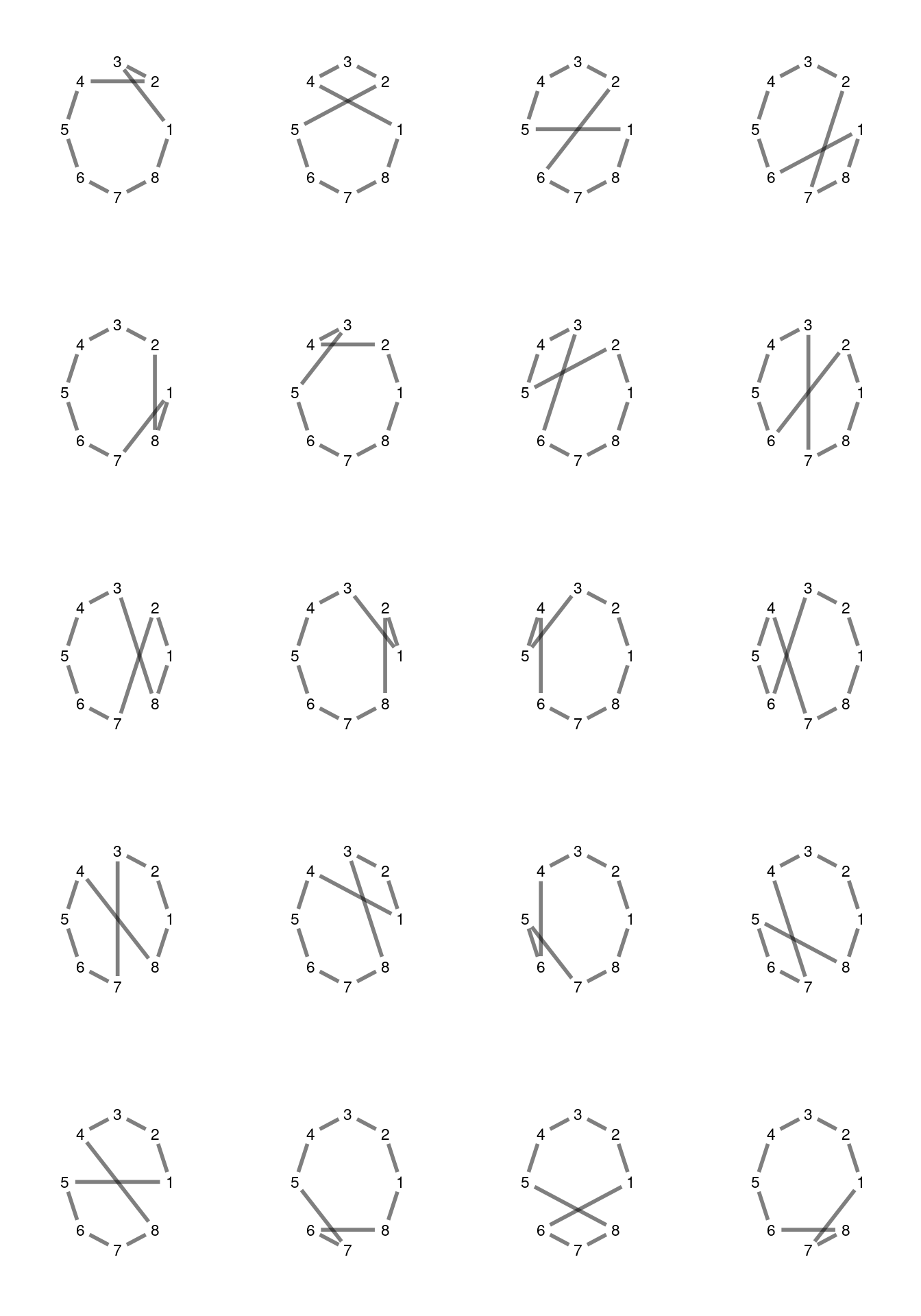
## [1] 1 2 3 4 6 5In the following figure, I am presenting the twenty 2-opt moves for a TSP instance of size eight.
Value of Solution for 2-opt Moves
In a local search algorithm like simulated annealing or tabu search, we need to perform many evaluations of the total distance of a solution, so it is relevant to calculate them in a fast way. Let’s illustrate how to do this with a distance matrix D of a TSP instance of size n = 8.
points <- function(n){
  df <- data.frame(x = sample(1:(2*n), n),
                   y = sample(1:(2*n), n))
  return(df)
}

n <- 8
set.seed(1111)
D <- dist(points(n), method = "manhattan", upper = TRUE) |> as.matrix()
The TSP() function calculates the value of a solution in a fast way.
TSP <- function(D, sol) sum(D[cbind(sol, c(sol[-1], sol[1]))])If we look again at the first picture, we observe that when we perform a 2-opt move, we remove two edges and add two new ones. So substracting and adding edge distances can be used to calculate objective function faster.
tsp_dist_2opt <- function(D, fit, sol, i, j, n){
  if(j == n)
    new_sol <- fit + D[sol[i-1], sol[j]] + D[sol[i], sol[1]] - D[sol[i-1], sol[i]] - D[sol[j], sol[1]]
  else
    new_sol <- fit +  D[sol[i-1], sol[j]] + D[sol[i], sol[j+1]] - D[sol[i-1], sol[i]] - D[sol[j], sol[j+1]]

  return(new_sol)
}
Let’s check if the function works. We start calculating the total distance of a solution sol.
set.seed(55)
sol <- c(1, sample(2:n, n-1))
sol
## [1] 1 7 3 5 4 2 6 8fit <- TSP(D, sol)
fit## [1] 98Now we generate a new solution with the \((3,6)\) move, and compare the result obtained in the two ways.
new_sol <- move_2opt(sol, 3, 6, 8)
new_sol
## [1] 1 7 2 4 5 3 6 8TSP(D, new_sol) ## [1] 90tsp_dist_2opt(D, fit, sol, 3, 6, 8)## [1] 90We observe that both functions lead to the same result.
Exploring a 2-opt Neighbourhood
We can use purrr:pmap() on the table of 2-opt moves to evaluate the value of cycle of each move, and find the best move arranging the table.
moves |>
  mutate(new_sol = pmap_dbl(moves, ~ tsp_dist_2opt(D, fit, sol, .x, .y, n))) |>
  arrange(new_sol, i)
## i j new_sol
## 1 3 5 82
## 2 4 6 86
## 3 4 7 86
## 4 5 7 86
## 5 3 6 90
## 6 3 8 92
## 7 5 8 92
## 8 6 8 96
## 9 5 6 98
## 10 2 7 100
## 11 3 4 100
## 12 6 7 100
## 13 2 5 102
## 14 3 7 102
## 15 4 5 102
## 16 2 4 104
## 17 2 6 106
## 18 2 3 110
## 19 7 8 110
## 20 4 8 114In this case, we observe that the best move for this solution is \((3,5)\), which reduces total cycle value from 98 to 82.
Session Info
## R version 4.5.0 (2025-04-11)
## Platform: x86_64-pc-linux-gnu
## Running under: Linux Mint 21.1
##
## Matrix products: default
## BLAS:   /usr/lib/x86_64-linux-gnu/blas/libblas.so.3.10.0
## LAPACK: /usr/lib/x86_64-linux-gnu/lapack/liblapack.so.3.10.0  LAPACK version 3.10.0
##
## locale:
##  [1] LC_CTYPE=es_ES.UTF-8       LC_NUMERIC=C
##  [3] LC_TIME=es_ES.UTF-8        LC_COLLATE=es_ES.UTF-8
##  [5] LC_MONETARY=es_ES.UTF-8    LC_MESSAGES=es_ES.UTF-8
##  [7] LC_PAPER=es_ES.UTF-8       LC_NAME=C
##  [9] LC_ADDRESS=C               LC_TELEPHONE=C
## [11] LC_MEASUREMENT=es_ES.UTF-8 LC_IDENTIFICATION=C
##
## time zone: Europe/Madrid
## tzcode source: system (glibc)
##
## attached base packages:
## [1] stats     graphics  grDevices utils     datasets  methods   base
##
## other attached packages:
## [1] patchwork_1.3.0 gridExtra_2.3   ggraph_2.2.1    ggplot2_3.5.2
## [5] tidygraph_1.3.1 purrr_1.0.4
##
## loaded via a namespace (and not attached):
##  [1] viridis_0.6.5      sass_0.4.10        generics_0.1.3     tidyr_1.3.1
##  [5] blogdown_1.21      digest_0.6.37      magrittr_2.0.3     evaluate_1.0.3
##  [9] grid_4.5.0         bookdown_0.43      fastmap_1.2.0      jsonlite_2.0.0
## [13] ggrepel_0.9.6      viridisLite_0.4.2  scales_1.3.0       tweenr_2.0.3
## [17] jquerylib_0.1.4    cli_3.6.4          rlang_1.1.6        graphlayouts_1.2.2
## [21] polyclip_1.10-7    munsell_0.5.1      withr_3.0.2        cachem_1.1.0
## [25] yaml_2.3.10        tools_4.5.0        memoise_2.0.1      dplyr_1.1.4
## [29] colorspace_2.1-1   vctrs_0.6.5        R6_2.6.1           lifecycle_1.0.4
## [33] MASS_7.3-65        pkgconfig_2.0.3    pillar_1.10.2      bslib_0.9.0
## [37] gtable_0.3.6       glue_1.8.0         Rcpp_1.0.14        ggforce_0.4.2
## [41] xfun_0.52          tibble_3.2.1       tidyselect_1.2.1   rstudioapi_0.17.1
## [45] knitr_1.50         farver_2.1.2       htmltools_0.5.8.1  igraph_2.1.4
## [49] labeling_0.4.3     rmarkdown_2.29     compiler_4.5.0
Post updated on 2025-06-02.