Neighbourhood definition is a key step to turn metaheuristics like tabu search or simulated annealing into algorithms to solve combinatorial optimization problems. For routing problems like the travelling salesman problem (TSP), the 2-opt move is a natural move to establish a neighbourhood definition. The 2-opt move consists of picking a pair of non contiguous edges, and rearrange the connections between the four nodes of the two edges.
Im this post, I will use two small instances of the TSP from TSPLIB to evaluate tabu search and simulated annealing heuristics based on 2-opt moves. The algorithms use the tidyverse for data handling, and I also will use it for plotting algorithm evolution.
library(tidyverse)The code for the instances is in a gist file on GitHub:
devtools::source_gist("https://gist.github.com/jmsallan/913494f5495ea2ab7ece4ed131a3d314")## ℹ Sourcing gist "913494f5495ea2ab7ece4ed131a3d314"
## ℹ SHA-1 hash of file is "d1117e1dd9823301bf7cb056b1dbf3940bc34363"The selected instances are gr24 and gr48. The optimum value of the solution for these instances is:
tsp_dist(gr24$D, gr24$opt.tour)## [1] 1272tsp_dist(gr48$D, gr48$opt.tour)## [1] 5046A first step to apply local search algorithms effectively is using the solution of a constructive heuristic as starting solution. Here I will be using the nearest neighbour heuristic, starting from node 1.
nn_gr24 <- nn_tsp(gr24$D)
nn_gr48 <- nn_tsp(gr48$D)

nn_gr24$fit
## [1] 1553nn_gr48$fit## [1] 6098For these two instances, the solutions obtained with the constructive heuristic are far from optimality.
Tabu Search
Let’s apply a tabu search algorithm to solve the gr24 instance. The tabu list size of 100 may seem long, but a neighbourhood of a solution for an instance of 24 nodes has 24*21/2 = 252 solution.
t1 <- Sys.time()
ts_gr24 <- tabu_2opt_tsp(instance = gr24$D, start_sol = nn_gr24$sol,
                         max_iter = 125, tabu_size = 100)
t2 <- Sys.time()
time_ts_gr24 <- difftime(t2, t1, units = "secs")
This run of the algorithm finds the optimal solution:
ts_gr24$fit## [1] 1272ts_gr24$sol## [1] 1 12 4 23 9 13 14 20 2 15 19 22 18 17 10 5 21 8 24 6 7 3 11 16tsp_dist(gr24$D, gr24$opt.tour)## [1] 1272gr24$opt.tour## [1] 16 11 3 7 6 24 8 21 5 10 17 22 18 19 15 2 20 14 13 9 23 4 12 1As this version of the tabu search is deterministic, all runs of the algorithm will always lead to the same solution. Here is the evolution of the algorithm, presenting the fitness of the current explored solution and the best solution found so far for each iteration.
custom_theme <- theme_minimal() +
  theme(legend.position = "bottom")

ts_gr24$track |>
  pivot_longer(-iter) |>
  ggplot(aes(iter, value, color = name)) +
  geom_line(linewidth = 0.8) +
  custom_theme +
  labs(x = NULL, y = NULL, title = "Tabu Search gr24") +
  scale_color_manual(name = "fitness", labels = c("best", "current"),
                     values = c("red", "#3399FF"))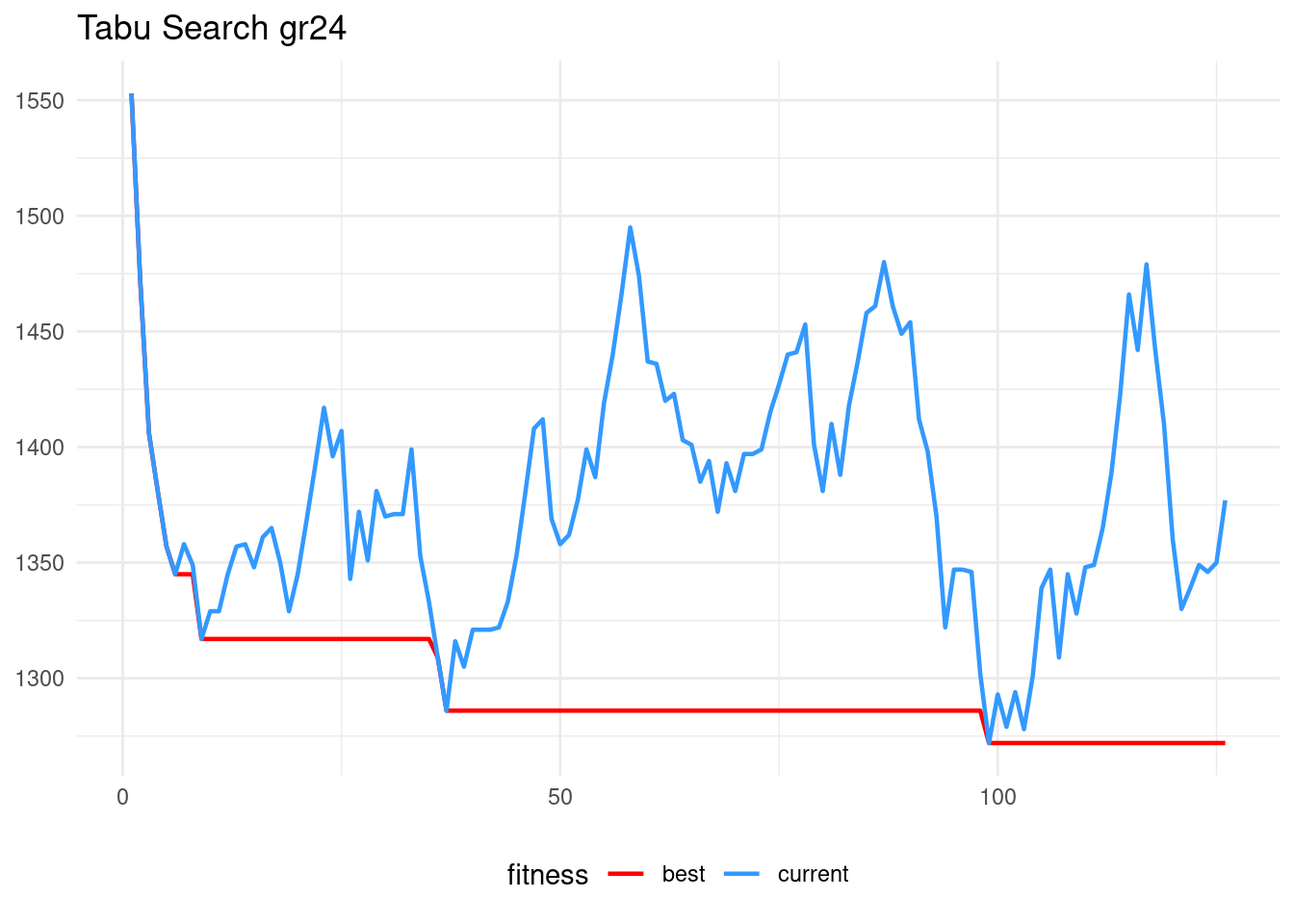
Let’s solve now the instance of 48 nodes gr48. The tabu list size is 200, and the size of the neighbourhood for this problem is 45*48/2 = 1080 solutions.
t1 <- Sys.time()
ts_gr48 <- tabu_2opt_tsp(instance = gr48$D, start_sol = nn_gr48$sol,
                         max_iter = 300, tabu_size = 200)
t2 <- Sys.time()
time_ts_gr48 <- difftime(t2, t1, units = "secs")
For this problem, the tabu search also finds the optimal solution.
ts_gr48$fit## [1] 5046ts_gr48$sol## [1] 1 13 48 16 11 36 26 6 14 9 32 27 17 21 22 8 33 5 31 12 10 15 24 37 47
## [26] 43 45 2 40 39 42 35 20 38 30 4 19 3 25 23 34 18 46 41 44 28 7 29tsp_dist(gr48$D, gr48$opt.tour)## [1] 5046gr48$opt.tour## [1] 29 7 28 44 41 46 18 34 23 25 3 19 4 30 38 20 35 42 39 40 2 45 43 47 37
## [26] 24 15 10 12 31 5 33 8 22 21 17 27 32 9 14 6 26 36 11 16 48 13 1This is the evolution of the tabu search for gr48.
ts_gr48$track |>
  pivot_longer(-iter) |>
  ggplot(aes(iter, value, color = name)) +
  geom_line(linewidth = 0.5) +
  custom_theme +
  labs(x = NULL, y = NULL, title = "Tabu Search gr48") +
  scale_color_manual(name = "fitness", labels = c("best", "current"),
                     values = c("red", "#3399FF"))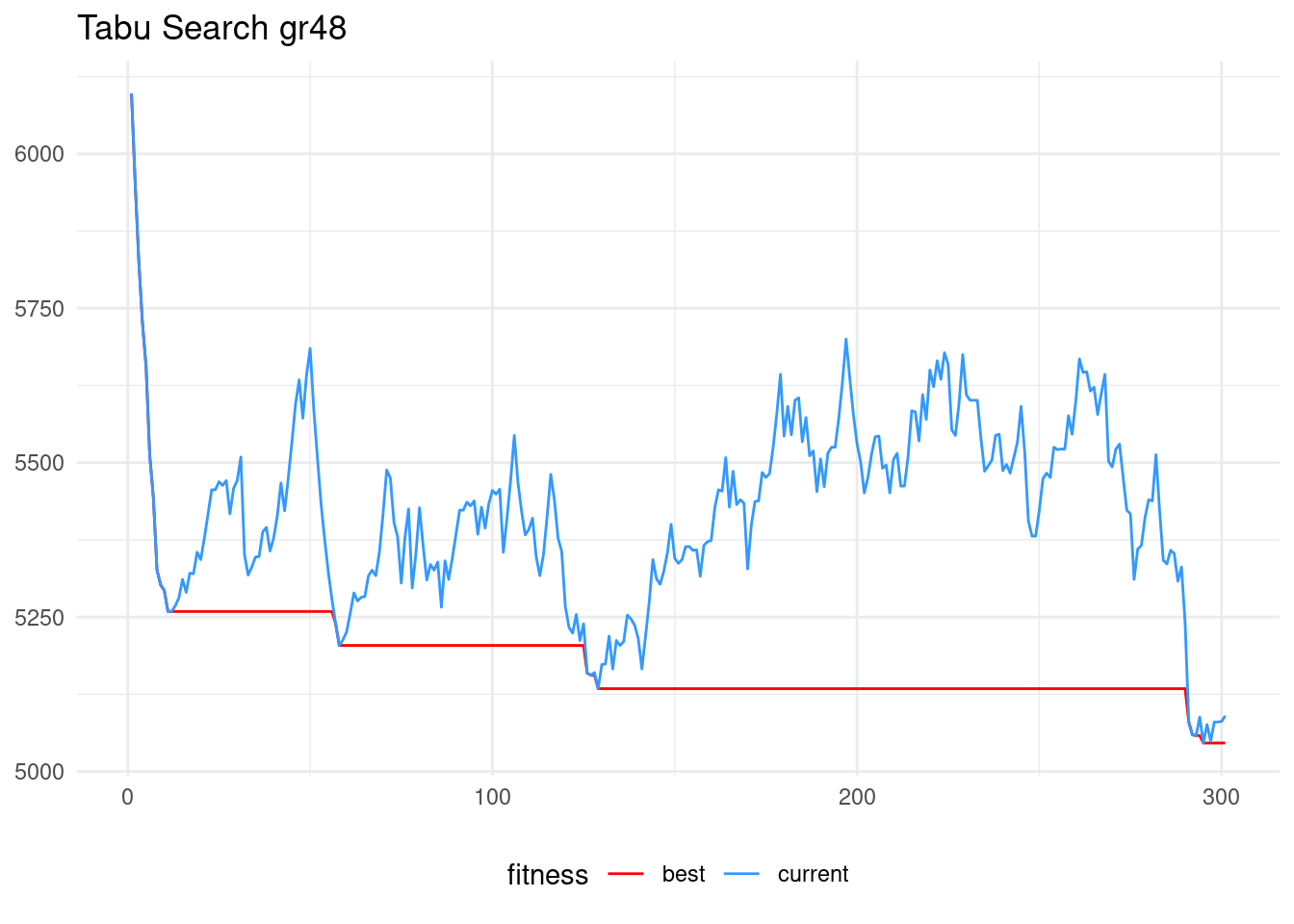
Simulated Annealing
As an alternative, we can try a simulated annealing heuristic. When comparing simulated annealing with tabu search, we must take into account that:
- Each iteration of the simulated annealing examines a single solution, so we must set the number of iterations so that both algoritjms examine roughly the same number of solutions.
- The simulated annealing is a stochastic algorithm, as it contains randomness, so two runs of the same algorithm may lead to different solutions.
For the gr24 instance, the tabu search had 125 runs, so to compare both algoirthms fairly the number of iterations of the simulated annealing should be of around 24x21x125/2 = 31500.
set.seed(1313)
t1 <- Sys.time()
sa_gr24 <- sa_2opt_tsp(instance = gr24$D, start_sol = nn_gr24$sol,
                       max_iter = 31500, alpha = 1 - 1e-03, p0 = 0.5)
t2 <- Sys.time()
time_sa_gr24 <- difftime(t2, t1, units = "secs")
The obtained solution is also optimal:
ts_gr24$fit## [1] 1272ts_gr24$sol## [1] 1 12 4 23 9 13 14 20 2 15 19 22 18 17 10 5 21 8 24 6 7 3 11 16tsp_dist(gr24$D, gr24$opt.tour)## [1] 1272gr24$opt.tour## [1] 16 11 3 7 6 24 8 21 5 10 17 22 18 19 15 2 20 14 13 9 23 4 12 1In the algorithm evolution plot, we can distinguish the exploration phase in the first iterations from the exploitation (refinement) phase of the last iterations.
sa_gr24$track |>
  pivot_longer(-iter) |>
  ggplot(aes(iter, value, color = name)) +
  geom_line(linewdith = 0.8) +
  custom_theme +
  labs(x = NULL, y = NULL, title = "Simulated Annealing gr24") +
  scale_color_manual(name = "fitness", labels = c("best", "current"),
                     values = c("red", "#3399FF"))
## Warning in geom_line(linewdith = 0.8): Ignoring unknown parameters: `linewdith`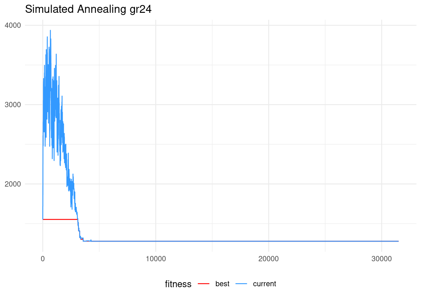
In stochastic algorithms, it can be convenient to run the algorithm several times, to account for solution variability. I am using map() to run the function ten times and store the result in a list.
set.seed(313)
runs_sa_gr24 <- map(1:10, ~  sa_2opt_tsp(instance = gr24$D, start_sol = nn_gr24$sol, max_iter = 31500, alpha = 1 - 1e-03, p0 = 0.5))
Once extracted the results, I use map_dbl() to extract the value of the fitness function
map_dbl(runs_sa_gr24, ~ .$fit)## [1] 1272 1335 1319 1278 1272 1342 1272 1317 1286 1279This sampling illustrates that, unlike tabu search, we are never sure of obtaining the same solution each time we run the algorithm. For this instance, we can see that variability is relatively low, and that it is frequent to reach the optimal solution.
Finally, let’s examine the simulated annealing algorithm for the instance of 48 nodes. This instance would be requiring 48x45x300/2 = 324800 runs.
set.seed(1313)
t1 <- Sys.time()
sa_gr48 <- sa_2opt_tsp(instance = gr48$D, start_sol = nn_gr48$sol,
                       max_iter = 324800, alpha = 1 - 1e-03, p0 = 0.5)
t2 <- Sys.time()
time_sa_gr48 <- difftime(t2, t1, units = "secs")
The obtained solution is near to the optimum, but does not reach optimality like tabu search.
sa_gr48$fit## [1] 5097sa_gr48$sol## [1] 1 29 7 28 44 41 25 3 19 4 30 38 20 35 42 39 40 2 45 43 23 34 46 18 47
## [26] 37 24 10 12 31 5 33 15 26 8 22 32 27 17 21 9 14 6 36 11 16 48 13tsp_dist(gr48$D, gr48$opt.tour)## [1] 5046gr24$opt.tour## [1] 16 11 3 7 6 24 8 21 5 10 17 22 18 19 15 2 20 14 13 9 23 4 12 1Regarding the evolution of the algorithm, the exploration phase is relatively shorter than in the 24 nodes instance. Changes in the alpha parameter (not shown here) do not show significant improvement of performance.
sa_gr48$track |>
  pivot_longer(-iter) |>
  ggplot(aes(iter, value, color = name)) +
  geom_line(linewidth = 0.8) +
  custom_theme +
  labs(x = NULL, y = NULL, title = "Simulated Annealing gr48") +
  scale_color_manual(name = "fitness", labels = c("best", "current"),
                     values = c("red", "#3399FF"))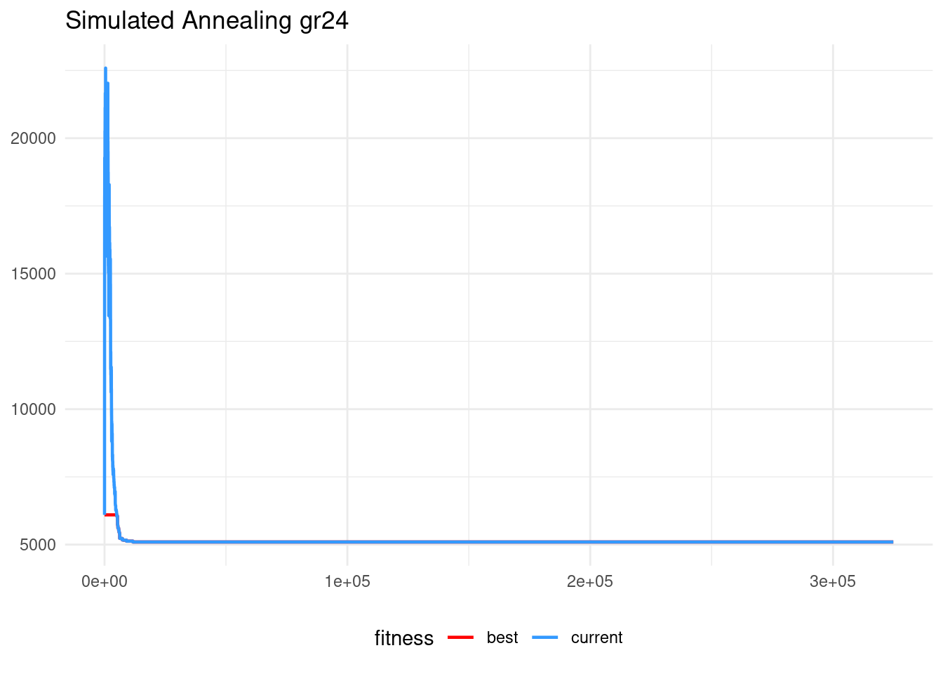
Comparing Algorithm Performance
Tabu search and simulated annealing are two local search metaheuristics for optimization of combinatorial problems. To obtain an heuristic for a specific problem, we need to define an adequate neighborhood for a solution. For routing problems like the travelling salesman problem, the 2-opt neighborhood is specially adequate.
I have used two instances of the TSP of 24 and 48 nodes from TSPLIB to test these heuristics. These instances can be considered small for the current state of the art of the TSP, but are still hard to handle for linear programming formulations.
The results are somewhat different for each instance. In gr24, both heuristics fins the optimal solution. It must be noted, though, that the results of the simulated annealing are different for each run. For this instance, an advantage of simulated annealing is time of execution:
time_ts_gr24## Time difference of 8.986598 secstime_sa_gr24## Time difference of 2.995294 secsIndeed, we observe that simulated annealing is faster than tabu search, with a similar number of evaluations of the objective function.
Regarding gr48, the time of execution of tabu search is smaller than simulated annealing.
time_ts_gr48## Time difference of 146.099 secstime_sa_gr48## Time difference of 290.9121 secsAs the tabu search finds the optimal solution while simulated annealing does not, we can conclude that tabu search is better than simulated annealing for instances of around 48 nodes. This conclusion, though, is pending of a more formal evaluation of hyperparameters of the simulated annealing algorithm.
We can also observe than the time required to reach a (nearly) optimal solution for gr48 is more than double than for gr24. This suggests that larger instances should be tackled with more elaborated, time consuming heuristics, like GRASP or iterated local search.
References
- 2-opt moves in the travelling salesman problem. https://jmsallan.netlify.app/blog/2-opt-moves-in-the-travelling-salesman-problem/
- gist with code of functions: https://gist.github.com/jmsallan/913494f5495ea2ab7ece4ed131a3d314
- TSPLIB http://comopt.ifi.uni-heidelberg.de/software/TSPLIB95/
Session Info
## R version 4.5.1 (2025-06-13)
## Platform: x86_64-pc-linux-gnu
## Running under: Linux Mint 21.1
##
## Matrix products: default
## BLAS:   /usr/lib/x86_64-linux-gnu/blas/libblas.so.3.10.0
## LAPACK: /usr/lib/x86_64-linux-gnu/lapack/liblapack.so.3.10.0  LAPACK version 3.10.0
##
## locale:
##  [1] LC_CTYPE=es_ES.UTF-8       LC_NUMERIC=C
##  [3] LC_TIME=es_ES.UTF-8        LC_COLLATE=es_ES.UTF-8
##  [5] LC_MONETARY=es_ES.UTF-8    LC_MESSAGES=es_ES.UTF-8
##  [7] LC_PAPER=es_ES.UTF-8       LC_NAME=C
##  [9] LC_ADDRESS=C               LC_TELEPHONE=C
## [11] LC_MEASUREMENT=es_ES.UTF-8 LC_IDENTIFICATION=C
##
## time zone: Europe/Madrid
## tzcode source: system (glibc)
##
## attached base packages:
## [1] stats     graphics  grDevices utils     datasets  methods   base
##
## other attached packages:
##  [1] lubridate_1.9.4 forcats_1.0.0   stringr_1.5.1   dplyr_1.1.4
##  [5] purrr_1.0.4     readr_2.1.5     tidyr_1.3.1     tibble_3.2.1
##  [9] ggplot2_3.5.2   tidyverse_2.0.0
##
## loaded via a namespace (and not attached):
##  [1] gtable_0.3.6      httr2_1.1.2       xfun_0.52         bslib_0.9.0
##  [5] htmlwidgets_1.6.4 devtools_2.4.5    remotes_2.5.0     gh_1.5.0
##  [9] tzdb_0.5.0        vctrs_0.6.5       tools_4.5.1       generics_0.1.3
## [13] curl_6.2.2        pkgconfig_2.0.3   lifecycle_1.0.4   farver_2.1.2
## [17] compiler_4.5.1    munsell_0.5.1     httpuv_1.6.16     htmltools_0.5.8.1
## [21] usethis_3.1.0     sass_0.4.10       yaml_2.3.10       pillar_1.10.2
## [25] later_1.4.2       jquerylib_0.1.4   urlchecker_1.0.1  ellipsis_0.3.2
## [29] cachem_1.1.0      sessioninfo_1.2.3 mime_0.13         tidyselect_1.2.1
## [33] digest_0.6.37     stringi_1.8.7     bookdown_0.43     labeling_0.4.3
## [37] fastmap_1.2.0     grid_4.5.1        colorspace_2.1-1  cli_3.6.4
## [41] magrittr_2.0.3    pkgbuild_1.4.8    withr_3.0.2       rappdirs_0.3.3
## [45] scales_1.3.0      promises_1.3.2    timechange_0.3.0  httr_1.4.7
## [49] rmarkdown_2.29    gitcreds_0.1.2    blogdown_1.21     hms_1.1.3
## [53] memoise_2.0.1     shiny_1.10.0      evaluate_1.0.3    knitr_1.50
## [57] miniUI_0.1.2      profvis_0.4.0     rlang_1.1.6       Rcpp_1.0.14
## [61] xtable_1.8-4      glue_1.8.0        pkgload_1.4.0     rstudioapi_0.17.1
## [65] jsonlite_2.0.0    R6_2.6.1          fs_1.6.6